Generalized additive models (GAM)
GAM models are currently experimental.
Introduction
A Generalized Additive Model (GAM) is a type of Generalized Linear Model (GLM) where the linear predictor has a linear relationship with predictor variables and smooth functions of predictor variables. H2O's GAM implementation is closely based on the approach described in "Generalized Additive Models: An Introduction with R, Texts in Statistical Science [1]" by Simon N. Wood. Another useful resource on GAMs can be found in "Generalized Additive Models" by T.J. Hastie and R.J. Tibshirani [2].
MOJO support
GAM supports importing and exporting MOJOs.
Defining a GAM model
Parameters are optional unless specified as required. GAM shares many GLM parameters.
Algorithm-specific parameters
-
bs: An array specifying the spline types for each GAM predictor. You must include one value for each GAM predictor. One of:
0(default) specifies cubic regression spline.1specifies thin plate regression with knots.2specifies monotone splines (or I-splines).3specifies NBSplineTypeI M-splines (which can support any polynomial order).
-
gam_columns: Required Include an array of column names representing the smoothing terms used for prediction. GAM will build a smoother for each specified column.
-
keep_gam_cols: Specify whether to save keys storing GAM columns. This option defaults to
False(disabled). -
knot_ids: A string array storing frame keys/IDs that contain knot locations. Specify one value for each GAM column specified in
gam_columns. -
num_knots: An array that specifies the number of knots for each predictor specified in
gam_columns. -
scale: An array specifying the smoothing parameter for GAM. If specified, must be the same length as
gam_columns. -
scale_tp_penalty_mat: Scale penalty matrix for thin plate smoothers. This option defaults to
False. -
splines_non_negative: (Applicable for I-spline or
bs=2only) Set this option toTrueif the I-splines are monotonically increasing (or monotonically non-decreasing). Set this option toFalseif the I-splines are monotonically decreasing (or monotonically non-increasing). If specified, this option must be the same size asgam_columns. Values for other spline types will be ignored. This option defaults toTrue(enabled). -
spline_orders: Order of I-splines (also known as monotone splines) and NBSplineTypeI M-splines used for GAM predictors. For I-splines, the
spline_orderswill be the same as the polynomials used to generate the splines. For M-splines, the polynomials will bespline_orders. For example,spline_orders=3for I-splines means a polynomial of order 3 will be used in the splines while for M-splines it means a polynomial of order 2 will be used. If specified, this option must be the same size asgam_columns. Values forbs=0orbs=1will be ignored. -
standardize_tp_gam_cols: Standardize thin plate predictor columns. This option defaults to
False. -
subspaces: List model parameters that can vary freely within the same subspace list, allowing the user to group model parameters with restrictions. If specified, the following parameters must have the same array dimsension:
gam_columnsnum_knotsscalebs
Here is an example specifying these parameters:
gam = H2OGeneralizedAdditiveEstimator(family='binomial',gam_columns=["C11", "C12", "C13", ["C14", "C15"]],knot_ids=[frameKnotC11.key, framKnotC12.key, frameKnotC13.key, frameKnotC145.key],bs=[0,2,3,1],standardize=True,lambda_=[0],alpha=[0],max_iterations=1,store_knot_locations=True)
Common parameters
-
auc_type: Set the default multinomial AUC type. Must be one of:
"AUTO"(default)"NONE""MACRO_OVR""WEIGHTED_OVR""MACRO_OVO""WEIGHTED_OVO"
-
early_stopping: Specify whether to stop early when there is no more relative improvement on the training or validation set. This option defaults to
True(enabled). -
export_checkpoints_dir: Specify a directory to which generated models will automatically be exported.
-
fold_assignment: (Applicable only if a value for
nfoldsis specified andfold_columnis not specified) Specify the cross-validation fold assignment scheme. One of:AUTO(default; usesRandom)RandomModulo(read more about Modulo)Stratified(which will stratify the folds based on the response variable for classification problems)
-
fold_column: Specify the column that contains the cross-validation fold index assignment per observation.
-
ignore_const_cols: Enable this option to ignore constant training columns as they provide no useful information. This option defaults to
True(enabled). -
ignored_columns: (Python only) Specify the column or columns to be excluded from the model.
-
keep_cross_validation_fold_assignment: Enable this option to preserve the cross-validation fold assignment. This option defaults to
False(disabled). -
keep_cross_validation_models: Specify whether to keep the cross-validated models. Keeping cross-validation models may consume significantly more memory in the H2O cluster. This option defaults to
True(enabled). -
keep_cross_validation_predictions: Specify whether to keep the cross-validation predictions. This option defaults to
False(disabled). -
max_active_predictors: Specify the maximum number of active predictors during computation. This value is used as a stopping criterium to prevent expensive model building with many predictors. This value defaults to
-1(unlimited). This default indicates that if theIRLSMsolver is used, the value ofmax_active_predictorsis set to5000, otherwise it is set to100000000. -
max_iterations: Specify the number of training iterations. This option defaults to
-1(unlimited). -
max_runtime_secs: Maximum allowed runtime in seconds for model training. Use
0(default) to disable. -
missing_values_handling: Choose how to handle missing values (one of:
Skip,MeanImputation(default), orPlugValues). -
model_id: Provide a custom name for the model to use as a reference. By default, H2O automatically generates a destination key.
-
nfolds: Specify the number of folds for cross-validation. The value can be
0(default) to disable or2. -
offset_column: Specify a column to use as the offset; the value cannot be the same as the
weights_column.Note: Offsets are per-row "bias values" that are used during model training. For Gaussian distributions, they can be seen as simple corrections to the response (
y) column. Instead of learning to predict the response (y-row), the model learns to predict the (row) offset of the response column. For other distributions, the offset corrections are applied in the linearized space before applying the inverse link function to get the actual response values. -
score_each_iteration: Enable this option to score during each iteration of the model training. This option defaults to
False(disabled). -
seed: Specify the random number generator (RNG) seed for algorithm components dependent on randomization. The seed is consistent for each H2O instance so that you can create models with the same starting conditions in alternative configurations. This option defaults to
-1(time-based random number). -
standardize: Specify whether to standardize the numeric columns to have a mean of zero and unit variance. Standardization is highly recommended; if you do not use standardization, the results can include components that are dominated by variables that appear to have larger variances relative to other attributes as a matter of scale, rather than true contribution. This option defaults to
False(disabled). -
stopping_metric: Specify the metric to use for early stopping. The available options are:
AUTO(default): (This defaults tologlossfor classification anddeviancefor regression)devianceloglossMSERMSEMAERMSLEAUC(area under the ROC curve)AUCPR(area under the Precision-Recall curve)lift_top_groupmisclassificationmean_per_class_error
-
stopping_rounds: Stops training when the option selected for
stopping_metricdoesn't improve for the specified number of training rounds, based on a simple moving average. To disable this feature, specify0(default).Note: If cross-validation is enabled:
- All cross-validation models stop training when the validation metric doesn't improve.
- The main model runs for the mean number of epochs.
- N+1 models may be off by the number specified for
stopping_roundsfrom the best model, but the cross-validation metric estimates the performance of the main model for the resulting number of epochs (which may be fewer than the specified number of epochs).
-
stopping_tolerance: Specify the relative tolerance for the metric-based stopping to stop training if the improvement is less than this value. This option defaults to
0.001. -
training_frame: Required Specify the dataset used to build the model.
-
validation_frame: Specify the dataset used to evaluate the model's accuracy.
-
weights_column: Specify a column to use for the observation weights, which are used for bias correction. The specified
weights_columnmust be included in the specifiedtraining_frame.Python only: To use a weights column when passing an H2OFrame to
xinstead of a list of column names, the specifiedtraining_framemust contain the specifiedweights_column.Note: Weights are per-row observation weights and do not increase the size of the data frame. This is typically the number of times a row is repeated, but non-integer values are supported as well. During training, rows with higher weights matter more due to the larger loss function pre-factor.
-
x: Specify a vector containing the names or indices of the predictor variables to use when building the model. If
xis missing, then no predictors will be used. -
y: Required Specify the column to use as the dependent variable.
- For a regression model, this column must be numeric (Real or Int).
- For a classification model, this column must be categorical (Enum or String). If the family is
Binomial, the dataset must contain two levels.
A simple linear model
For observations, with response variable , where is an observation on random variable . and . Assuming a linear relationship between the predictor variables and the response, the relationship between and is:
and are unknown parameters, are i.i.d zero mean variables with variances . We can estimate using GLM.
A simple linear GAM model
Using the same observations as in the previous A Simple Linear Model section, a linear GAM model can be:
Again, is an unknown parameter vector that can also be estimated using GLM. This can be done by using as the predictor variables instead of . We are essentially estimating using a set of basis functions:
where is the number of basis functions used. Note that for each predictor variable, we can decide the types and number of basis functions that we want to use to generate best GAM.
Understanding simple piecewise linear basis functions
To comprehend the role of basis functions, let's take a look at a linear tent function. This will help us understand how piecewise basis functions work.
When working with piecewise basis functions, it's crucial to pay attention to the points where the function's derivative discontinuities occur. These points are where the linear pieces connect, and they are known as knots. We denote these knots by . And suppose that the knots are sorted, meaning that .
For , the basis function defined as:
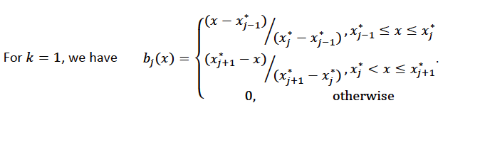
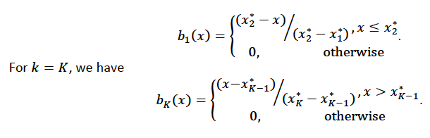
This function helps us understand how the linear pieces join together and interact with each other.
Using piecewise tent functions to approximate a single predictor variable
To illustrate how we can use the piecewise tent functions to approximate a predictor variable, let's take an example where the predictor value ranges from 0.0 to 1.0.:
We will use 10 piecewise tent functions, with K = 10. The knots will be located at 0, 1/9, 2/9, 3/9, …, 8/9, 1. The figure below shows the basis function values, which overlap with their neighbors except for the first and last basis functions.
![Ten piecewise tent basis functions over [0, 1]](/h2o-3-secure/assets/images/gam_piecewise_tent_basis-373efb34010dd9dc62006d4cc51d87e0.png)
For simplicity, assume we have 21 predictor values uniformly distributed between 0 and 1, with values of 0, 0.05, 0.1, 0.15, …, 1.0. Our goal is to convert each into a set of 10 basis function values. For every value, 10 values correspond to each of the basis functions.
For the predictor value at 0 (), the only relevant basis function is the first one. All other basis functions contribute 0 to the predictor value. Thus, for the vector representing all basis functions has these values: {1, 0, 0, 0, 0, 0, 0, 0, 0, 0}. This is because the first basis function value is 1 at :
For predictor value 0.05, only the first and second basis functions contribute, while the others are 0 at 0.05. The value of the first basis function is 0.55. which can be obtained by substituting in the first basis function:
The value of the second basis function at 0.05 is 0.45. Note Substitute to the second basis function
Hence, for , the vector corresponding to all basis function is {0.55,0.45,0,0,0,0,0,0,0,0}.
We have calculated the expanded basis function vector for all predictor values, and they can be found in following table.
| 0 | 1 | 0 | 0 | 0 | 0 | 0 | 0 | 0 | 0 | 0 |
| 0.05 | 0.55 | 0.45 | 0 | 0 | 0 | 0 | 0 | 0 | 0 | 0 |
| 0.1 | 0.1 | 0.9 | 0 | 0 | 0 | 0 | 0 | 0 | 0 | 0 |
| 0.15 | 0 | 0.65 | 0.35 | 0 | 0 | 0 | 0 | 0 | 0 | 0 |
| 0.2 | 0 | 0.2 | 0.8 | 0 | 0 | 0 | 0 | 0 | 0 | 0 |
| 0.25 | 0 | 0 | 0.75 | 0.25 | 0 | 0 | 0 | 0 | 0 | 0 |
| 0.3 | 0 | 0 | 0.3 | 0.7 | 0 | 0 | 0 | 0 | 0 | 0 |
| 0.35 | 0 | 0 | 0 | 0.85 | 0.15 | 0 | 0 | 0 | 0 | 0 |
| 0.4 | 0 | 0 | 0 | 0.4 | 0.6 | 0 | 0 | 0 | 0 | 0 |
| 0.45 | 0 | 0 | 0 | 0 | 0.95 | 0.05 | 0 | 0 | 0 | 0 |
| 0.5 | 0 | 0 | 0 | 0 | 0.5 | 0.5 | 0 | 0 | 0 | 0 |
| 0.55 | 0 | 0 | 0 | 0 | 0.05 | 0.95 | 0 | 0 | 0 | 0 |
| 0.6 | 0 | 0 | 0 | 0 | 0 | 0.6 | 0.4 | 0 | 0 | 0 |
| 0.65 | 0 | 0 | 0 | 0 | 0 | 0.15 | 0.85 | 0 | 0 | 0 |
| 0.7 | 0 | 0 | 0 | 0 | 0 | 0 | 0.7 | 0.3 | 0 | 0 |
| 0.75 | 0 | 0 | 0 | 0 | 0 | 0 | 0.25 | 0.75 | 0 | 0 |
| 0.8 | 0 | 0 | 0 | 0 | 0 | 0 | 0 | 0.8 | 0.2 | 0 |
| 0.85 | 0 | 0 | 0 | 0 | 0 | 0 | 0 | 0.35 | 0.65 | 0 |
| 0.9 | 0 | 0 | 0 | 0 | 0 | 0 | 0 | 0 | 0.9 | 0.1 |
| 0.95 | 0 | 0 | 0 | 0 | 0 | 0 | 0 | 0 | 0.45 | 0.55 |
| 1 | 0 | 0 | 0 | 0 | 0 | 0 | 0 | 0 | 0 | 1 |
Spline functions
Natural cubic splines are proven to be the smoothest interpolators, as shown in [2]. Given a set of points where , the natural cubic spline, , interpolates these points using sections of cubic polynomial for each . These sections are joined together so that the entire spline is continuous to the second derivative, with and . To ensure a smooth function, a penalty function can be added to the objective function being optimized. This penalty is based on the idea that a function's second derivative measures gradient change, and a higher second derivative magnitude indicates more wriggling.
Cubic regression splines
Implemented based on [1], cubic regression splines are used for a single predictor variable. This approach defines the splines in terms of their values at the knots. A cubic spline function, , with knots, , is defined using and .
The splines can be expressed as:
where:
To ensure smooth fitting functions at the knots, the spline must be continuous to the second derivative at and have zero second derivative at and . It can be shown that , where
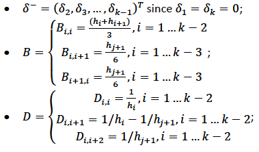
Let and let
The spline can be rewritten entirely in terms of as
which can be expressed as where are the basis functions and are the unknown parameters that can be estimated using GLM. Additionally, the penalty term added to the final objective function can be derived as:
where
For linear regression models, the final objective function to minimize is
Note that the user will choose using grid search. In future releases, cross-validation may be used to automatically select .
At this point, GLM can be called, but the contribution of the penalty term to the gradient and Hessian calculation still needs to be added.
Thin plate regression splines
For documentation on thin plate regression splines, refer to Thin plate regression splines.
Monotone splines
We have implemented I-splines, which are used as monotone splines. Monotone splines do not support multinomial or ordinal families. To specify the monotone spline, you need to set bs = 2 and specify spline_orders, which will be equal to the polynomials used to generate the splines. B-splines:
B-splines are generated using a recursive formula over a set of knots that covers the input range of interest. The number of basis functions for B-splines over the original knots is , where is the number of knots without duplication and is the spline order.
Using knotes over the range of inputs of interest from to , an order 1 B-spline is defined as [4]:
Extending the number of knots
To generate higher order splines, you have to extend the original knots over the range of inputs of interest. You do this by adding knots of value to the front of the knots and knots of value to the end of the knots. The new duplication will look like:
where:
- and are the duplicates.
The formula we used to calculate the number of basis functions over the original knots is:
where:
- is the number of knots over the input range without duplication
- is the order of the spline
M-splines:
M-splines serve two functions: they are part of the construction of I-splines and they are normal (non-monotonic) splines that are implemented separate of the monotone spline as part of the GAM toolbox. You must set bs = 3 for M-splines. spline_orders must also be set where the polynomials used to generate the splines will be equal to spline_orders-1. If you set spline_orders = 1 then you must set num_knots >= 3.
The B-spline function can be normalized and denoted as where it has an integration of 1 over the range of interest and is non-zero. This is the normalized B-spline Type I, and it is defined as:
with the property .
You can derive using the following recursive formula:
Note that is defined over the same knot sequence as the original B-spline, and the number of splines is the same as the number of B-splines over the same known sequence.
N-splines:
The N-splines are normalized to have a summation of 1 when as . is the normalized B-spline Type II in this implementation. The N-splines share the same knot sequence with the original M-spline and B-spline. The N-spline can be derived from the M-spline or the B-spline using:
Or, you can use the recursive formula where higher order N-splines can be derived from two lower order N-splines:
I-splines:
I-splines are used to build monotone spline functions by restricting the gamified column coefficients to be 0. They are constructed using the N-splines.
Penalty Matrix
The objective function used to derive the coefficients for regression is:
The second derivative of all basis functions is defined as:
where the penalty matrix () for I-spline is defined as:
Element at row and column of is
Derivative of M-splines
The penalty matrix written in terms of the second derivative of M-spline as:
Instead of using the recursive expression, look at the coefficients associated with , take the second derivative, and go from there. This is the procedure to use:
- generate the coefficients of ;
- implement multiplication of coefficients of . Due to the commutative property, , so you only need to perform the multiplication once and the is symmetrical;
- implement the integration of by easy integration of the coefficients.
General GAM
In a generalized additive model (GAM), using the GLM jargon, the link function can be constructed using a mixture of predictor variables and smooth functions of predictor variables as follows:
This is the GAM we implemented in H2O. However, with multiple predictor variables in any form, we need to resolve the identifiability problems by adding identifiability constraints.
Identifiability constraints
Consider GAM with multiple predictor smooth functions like the following:
The model now contains more than one function introduces an identifiability problem: an are each only estimable to within an additive constant. This is due to the fact that . Hence, identifiability constraints have to be imposed on the model before fitting to avoid the identifiability problem. The following sum-to-zero constraints are implemented in H2O:
where 1 is a column vector of 1, and is the column vector containing . To apply the sum-to-zero constraints, a Householder transform is used. Refer to [1] for details. This transform is applied to each basis function of any predictor column we choose on its own.
Note: this does not apply to monotone splines because the coefficients for these splines must be .
Sum-to-zero constraints implementation
Let be the model matrix that contain the basis functions of one predictor variable, the sum-to-zero constraints required that
where contains the coefficients relating to the basis functions of that particular predictor column. The idea is to create a matrix such that , then for any . To see how this works, let's go through the following derivations:
- With , we are looking at
- Let , then the QR decomposition of where is of size , is of size , is the size of
- Substitute everything back to since
Generating the Z matrix
One Householder reflection is used to generate the matrix. To create the matrix, we need to calculate the QR decomposition of Since is of size , the application of one householder reflection will generate where is of size . This implies that , since the householder reflection matrix is symmetrical. Hence, computing is equivalent to computing and dropping the first column.
Generating the Householder reflection matrix H
Let and , then and .
Estimation of GAM coefficients with identifiability constraints
The following procedure is used to estimate the GAM coefficients:
- Generating matrix for each predictor column that uses smoothe functions
- Generate new model matrix for each predictor column smooth function as , new penalty function .
- Call GLM using model matrix , penalty function to get coefficient estimates of
- Convert to using and performing scoring with and the original model matrix .
Examples
Below are simple examples showing how to use GAM in R and Python.
General GAM
- R
- Python
library(h2o)
h2o.init()

# create frame knots
knots1 <- c(-1.99905699, -0.98143075, 0.02599159, 1.00770987, 1.99942290)
frame_Knots1 <- as.h2o(knots1)
knots2 <- c(-1.999821861, -1.005257990, -0.006716042, 1.002197392, 1.999073589)
frame_Knots2 <- as.h2o(knots2)
knots3 <- c(-1.999675688, -0.979893796, 0.007573327, 1.011437347, 1.999611676)
frame_Knots3 <- as.h2o(knots3)

# import the dataset
h2o_data <- h2o.importFile("https://s3.amazonaws.com/h2o-public-test-data/smalldata/glm_test/multinomial_10_classes_10_cols_10000_Rows_train.csv")

# Convert the C1, C2, and C11 columns to factors
h2o_data["C1"] <- as.factor(h2o_data["C1"])
h2o_data["C2"] <- as.factor(h2o_data["C2"])
h2o_data["C11"] <- as.factor(h2o_data["C11"])

# split into train and test sets
splits <- h2o.splitFrame(data = h2o_data, ratios = 0.8)
train <- splits[[1]]
test <- splits[[2]]

# Set the predictor and response columns
predictors <- colnames(train[1:2])
response <- 'C11'

# specify the knots array
numKnots <- c(5, 5, 5)

# build the GAM model
gam_model <- h2o.gam(x = predictors,
                     y = response,
                     training_frame = train,
                     family = 'multinomial',
                     gam_columns = c("C6", "C7", "C8"),
                     scale = c(1, 1, 1),
                     num_knots = numKnots,
                     knot_ids = c(h2o.keyof(frame_Knots1), h2o.keyof(frame_Knots2), h2o.keyof(frame_Knots3)))

# get the model coefficients
coefficients <- h2o.coef(gam_model)

# generate predictions using the test data
pred <- h2o.predict(object = gam_model, newdata = test)
import h2o
from h2o.estimators.gam import H2OGeneralizedAdditiveEstimator
h2o.init()

# create frame knots
knots1 = [-1.99905699, -0.98143075, 0.02599159, 1.00770987, 1.99942290]
frameKnots1 = h2o.H2OFrame(python_obj=knots1)
knots2 = [-1.999821861, -1.005257990, -0.006716042, 1.002197392, 1.999073589]
frameKnots2 = h2o.H2OFrame(python_obj=knots2)
knots3 = [-1.999675688, -0.979893796, 0.007573327,1.011437347, 1.999611676]
frameKnots3 = h2o.H2OFrame(python_obj=knots3)

# import the dataset
h2o_data = h2o.import_file("https://s3.amazonaws.com/h2o-public-test-data/smalldata/glm_test/multinomial_10_classes_10_cols_10000_Rows_train.csv")

# convert the C1, C2, and C11 columns to factors
h2o_data["C1"] = h2o_data["C1"].asfactor()
h2o_data["C2"] = h2o_data["C2"].asfactor()
h2o_data["C11"] = h2o_data["C11"].asfactor()

# split into train and validation sets
train, test = h2o_data.split_frame(ratios = [.8])

# set the predictor and response columns
y = "C11"
x = ["C1","C2"]

# specify the knots array
numKnots = [5,5,5]

# build the GAM model
h2o_model = H2OGeneralizedAdditiveEstimator(family='multinomial',
                                            gam_columns=["C6","C7","C8"],
                                            scale=[1,1,1],
                                            num_knots=numKnots,
                                            knot_ids=[frameKnots1.key, frameKnots2.key, frameKnots3.key])
h2o_model.train(x=x, y=y, training_frame=train)

# get the model coefficients
h2oCoeffs = h2o_model.coef()

# generate predictions using the test data
pred = h2o_model.predict(test)
GAM using monotone splines
- R
- Python
# Import the GLM test data:
gam_test = h2o.importFile("https://s3.amazonaws.com/h2o-public-test-data/smalldata/glm_test/binomial_20_cols_10KRows.csv")

# Split into train and validation sets:
splits <- h2o.splitFrame(data = gam_test, ratios = 0.8)
train <- splits[[1]]
test <- splits[[2]]

# Set the factors, predictors, and response:
gam_test["C1"] <- as.factor(gam_test["C1"])
gam_test["C2"] <- as.factor(gam_test["C2"])
gam_test["C21"] <- as.factor(gam_test["C21"])
predictors <- c("C1","C2")
response <- "C21"

# Build and train the model using spline order:
monotone_model <- h2o.gam(x = predictors, y = response,
                          training_frame = train,
                          family = 'binomial',
                          gam_columns = c("C11", "C12", "C13"),
                          scale = c(0.001, 0.001, 0.001),
                          bs = c(0, 2, 2),
                          num_knots = c(3, 4, 5),
                          spline_orders = c(2, 3, 4))

# Generate predictions using the test data:
pred <- h2o.predict(object = monotone_model, newdata = test)
# Import the GLM test data:
gam_test = h2o.import_file("https://s3.amazonaws.com/h2o-public-test-data/smalldata/glm_test/binomial_20_cols_10KRows.csv")

# Split into train and validation sets:
train, test = gam_test.split_frame(ratios = [.8])

# Set the factors, predictors, and response:
gam_test["C1"] = gam_test["C1"].asfactor()
gam_test["C2"] = gam_test["C2"].asfactor()
gam_test["C21"] = gam_test["C21"].asfactor()
predictors = ["C1","C2"]
response = "C21"

# Build and train your model using spline order:
monotone_model = H2OGeneralizedAdditiveEstimator(family="binomial",
                                                 gam_columns=["C11", "C12", "C13"],
                                                 scale=[0.001, 0.001, 0.001],
                                                 bs=[0,2,2],
                                                 spline_orders=[2,3,4],
                                                 num_knots=[3,4,5])
monotone_model.train(x=predictors, y=response, training_frame=train)

# Generate predictions using the test data:
pred = monotone_model.predict(test)
GAM using M-splines
- R
- Python
# Import the GLM test data set:
gam_test = h2o.importFile("https://s3.amazonaws.com/h2o-public-test-data/smalldata/glm_test/binomial_20_cols_10KRows.csv")

# Set the factors, predictors, and response:
gam_test["C1"] <- as.factor(gam_test["C1"])
gam_test["C2"] <- as.factor(gam_test["C2"])
gam_test["C21"] <- as.factor(gam_test["C21"])
predictors <- c("C1","C2")
response <- "C21"

# Split into train and validation sets:
splits <- h2o.splitFrame(data = gam_test, ratios = 0.8)
train <- splits[[1]]
test <- splits[[2]]

# Build and train the model using spline order:
mspline_model <- h2o.gam(x = predictors,
                         y = response,
                         training_frame = train,
                         family = "binomial",
                         gam_columns = c("C11", "C12", "C13"),
                         scale = c(0.001, 0.001, 0.001),
                         bs = c(2, 0, 3),
                         spline_orders = c(10, -1, 10),
                         num_knots = c(3, 4, 5))
# Retrieve the coefficients:
h2o.coef(mspline_model)
# Import the GLM test data set:
gam_test = h2o.import_file("https://s3.amazonaws.com/h2o-public-test-data/smalldata/glm_test/binomial_20_cols_10KRows.csv")

# Set the factors, predictors, and response:
gam_test["C1"] = gam_test["C1"].asfactor()
gam_test["C2"] = gam_test["C2"].asfactor()
gam_test["C21"] = gam_test["C21"].asfactor()
predictors = ["C1","C2"]
response = "C21"

# Split into train and validation sets:
train, test = gam_test.split_frame(ratios = [.8])

# Build and train your model using spline order:
mspline_model = H2OGeneralizedAdditiveEstimator(family="binomial",
                                                gam_columns=["C11", "C12", "C13"],
                                                scale=[0.001, 0.001, 0.001],
                                                bs=[2,0,3],
                                                spline_orders=[10,-1,10],
                                                num_knots=[3,4,5])
mspline_model.train(x=predictors, y=response, training_frame=train)

# Retrieve the coefficients:
coef = mspline_model.coef()
print(coef)
References
- Simon N. Wood, Generalized Additive Models: An Introduction with R, Texts in Statistical Science, CRC Press, Second Edition.
- T.J. Hastie, R.J. Tibshirani, Generalized Additive Models, Chapman and Hall, First Edition, 1990.
- Lecture 7 Divided Difference Interpolation Polynomial by Professor R.Usha, Department of Mathematics, IITM, https://www.youtube.com/watch?v=4m5AKnseSyI .
- Carl De Boor et. al., ON CALCULATING WITH B-SPLINES II. INTEGRATION, ResearchGate Article, January 1976.
- J.O. Ramsay, “Monotone Regression Splines in Action”, Statistical Science, 1988, Vol. 3, No. 4, 425-461.
- Submit and view feedback for this page
- Send feedback about H2O-3 Secure to cloud-feedback@h2o.ai