Generalized linear model (GLM)

Introduction

Generalized Linear Models (GLM) estimate regression models for outcomes following exponential distributions. In addition to the Gaussian (that is, normal) distribution, these include Poisson, binomial, and gamma distributions. Each serves a different purpose, and depending on distribution and link function choice, can be used either for prediction or classification.

The GLM suite includes:

• Gaussian regression
• Poisson regression
• Binomial regression (classification)
• Fractional binomial regression
• Quasibinomial regression
• Multinomial classification
• Gamma regression
• Ordinal regression
• Negative Binomial regression
• Tweedie distribution

MOJO support

GLM supports importing and exporting MOJOs.

Additional Resources

• GLM Booklet

Defining a GLM model

Parameters are optional unless specified as required.

Algorithm-specific parameters

• build_null_model: If set, will build a model with only the intercept. This option defaults to False.

• calc_like: Specify whether to return likelihood function value for HGLM or normal GLM. Setting this option to True while disabling HGLM will enable the calculation of the full log likelihood and full AIC. This option defaults to False (disabled).

• control_variables: Specify control variables which will be disabled for metric calculation and during scoring. This feature is experimental.

• custom_metric_func: Specify a custom evaluation function.

• dispersion_epsilon: If changes in dispersion parameter estimation or loglikelihood value is smaller than dispersion_epsilon, this will break out of the dispersion parameter estimation loop using maximum likelihood. This option defaults to 0.0001.

• dispersion_learning_rate: (Applicable only when dispersion_parameter_method="ml") This value controls how much the dispersion parameter estimate will be changed when the calculated loglikelihood actually decreases with the new dispersion. In this case, instead of setting dispersion = dispersion + change, it is dispersion + dispersion_learning_rate $\times$ change. This option must be > 0 and defaults to 0.5.

• dispersion_parameter_method: Method used to estimate the dispersion factor for Tweedie, Gamma, and Negative Binomial only. Can be one of "pearson" (default), "deviance", or "ml".

• fix_dispersion_parameter: Only used for Tweedie, Gamma and Negative Binomial GLM. If enabled, this option will use the dispersion parameter in init_dispersion_parameter as the standard error and use it to calculate the p-values. This option defaults to False.

• generate_scoring_history: Generate the scoring history for the GLM model when enabled. This may significantly slow down the algorithm. When enabled, you will also be able to fetch the average objective and the negative log likelihood using their accessor functions: average_objective and negative_log_likelihood. This option defaults to False (disabled).

• generate_variable_inflation_factors: If enabled, this option generates the variable inflation factors for numerical predictors. This option defaults to False (disabled).

• init_dispersion_parameter: Initial value of dispersion factor before being estimated using either "pearson" or "ml". This option defaults to 1.0.

• interactions: Specify a list of predictor column indices to interact. All pairwise combinations will be computed for this list.

• interaction_pairs: When defining interactions, use this option to specify a list of pairwise column interactions (interactions between two variables). Note that this is different than interactions, which will compute all pairwise combinations of specified columns.

• max_iterations: For GLM, must be $\geq$ 1 to obtain a proper model (or -1 for unlimited which is the default setting). Setting it to 0 will only return the correct coefficient names and an empty model.

• max_iterations_dispersion: Control the maximum number of iterations in the dispersion parameter estimation loop using maximum likelihood. This option defaults to 1000000.

• rand_family: The Random Component Family specified as an array. You must include one family for each random component. Currently only rand_family=["gaussisan"] is supported.

• upload_custom_metric: Upload a custom metric into a running H2O cluster.

Shared GLM family parameters

GLM Family: Generalized Additive Models (GAM) ModelSelection ANOVA GLM Hierarchical Generalized Linear Model (HGLM)

• alpha: Specify the regularization distribution between L1 and L2. A value of 1 produces LASSO regression; a value of 0 produces Ridge regression. The default value of alpha is 0 when SOLVER = 'L-BFGS'; otherwise it is 0.5 to specify a mixing between LASSO and Ridge regression.

• beta_constraints: Specify a dataset to use beta constraints. The selected frame is used to constrain the coefficient vector to provide upper and lower bounds. The dataset must contain a "names" column with valid coefficient names.

• beta_epsilon: Converge if beta changes less than this value (using L-infinity norm). This only applies to IRLSM solver, and the value defaults to 0.0001.

• cold_start: Specify whether the model should be built from scratch. This parameter is only applicable when building a GLM model with multiple alpha/lambda values. If False and for a fixed alpha value, the next model with the next lambda value out of the lambda array will be built using the coefficients and the GLM state values of the current model. If True, the next GLM model will be built from scratch. The default value is False.

  note

  If an alpha array is specified and for a brand new alpha, the model will be built from scratch regardless of the value of cold_start.

• compute_p_values: Request computation of p-values. P-values can be computed with or without regularization. Setting remove_collinear_columns is recommended. H2O will return an error if p-values are requested and there are collinear columns and remove_collinear_columns flag is not enabled. Note that this option is not available for family="multinomial" or family="ordinal"; IRLSM solver required. This option defaults to False (disabled).

• family: Specify the model type.

  • If the family is gaussian, the response must be numeric (Real or Int).
  • If the family is binomial, the response must be categorical 2 levels/classes or binary (Enum or Int).
  • If the family is fractionalbinomial, the response must be a numeric between 0 and 1.
  • If the family is multinomial, the response can be categorical with more than two levels/classes (Enum).
  • If the family is ordinal, the response must be categorical with at least 3 levels.
  • If the family is quasibinomial, the response must be numeric.
  • If the family is poisson, the response must be numeric and non-negative (Int).
  • If the family is negativebinomial, the response must be numeric and non-negative (Int).
  • If the family is gamma, the response must be numeric and continuous and positive (Real or Int).
  • If the family is tweedie, the response must be numeric and continuous (Real) and non-negative.
  • If the family is AUTO (default),
    • and the response is Enum with cardinality = 2, then the family is automatically determined as binomial.
    • and the response is Enum with cardinality > 2, then the family is automatically determined as multinomial.
    • and the response is numeric (Real or Int), then the family is automatically determined as gaussian.

• gradient_epsilon: (For solver="L_BFGS" only) Specify a threshold for convergence. If the objective value (using the L-infinity norm) is less than this threshold, the model is converged. If lambda_search=True, then this value defaults to .0001. If lambda_search=False and lambda is equal to zero, then this value defaults to .000001. For any other value of lambda, this value defaults to .0001. This value defaults to -1.

• intercept: Specify whether to include a constant term in the model. This option defaults to True (enabled).

• lambda: Specify the regularization strength.

• lambda_min_ratio: Specify the minimum lambda to use for lambda search (specified as a ratio of lambda_max, which is the smallest $\lambda$ for which the solution is all zeros). This value defaults to -1 which indicates that if the number of observations is greater than the number of variables, then lambda_min_ratio is set to 0.0001; if the number of observations is less than the number of variables, then lambda_min_ratio is set to 0.01.

• lambda_search: Specify whether to enable lambda search, starting with lambda max (the smallest $\lambda$ that drives all coefficients to zero). If you also specify a value for lambda_min_ratio, then this value is interpreted as lambda min. If you do not specify a value for lambda_min_ratio, then GLM will calculate the minimum lambda. This option defaults to False (disabled).

• link: Specify a link function (one of: Identity, Family_Default (default), Logit, Log, Inverse, Tweedie, or Ologit).

  • If the family is Gaussian, then Identity, Log, and Inverse are supported.

  • If the family is Binomial, then Logit is supported.

  • If the family is Fractionalbinomial, then Logit is supported.

  • If the family is Poisson, then Log and Identity are supported.

  • If the family is Gamma, then Inverse, Log, and Identity are supported.

  • If the family is Tweedie, then only Tweedie is supported.

  • If the family is Multinomial, then only Family_Default is supported. (This defaults to multinomial.)

  • If the family is Quasibinomial, then only Logit is supported.

  • If the family is Ordinal, then only Ologit is supported

  • If the family is Negative Binomial, then Log and Identity are supported.

  • If the family is AUTO,

    • and a link is not specified, then the link is determined as Family_Default (defaults to the family to which AUTO is determined).

    • and a link is specified, the link is used so long as the specified link is compatible with the family to which AUTO is determined. Otherwise, an error message is thrown stating that AUTO for underlying data requires a different link and gives a list of possible compatible links.

    • The list of supported links for family = AUTO is:

      1. If the response is Enum with cardinality = 2, then Logit is supported.
      2. If the response is Enum with cardinality > 2, then only Family_Default is supported (this defaults to multinomial).
      3. If the response is numeric (Real or Int), then Identity, Log, and Inverse are supported.

• max_active_predictors: Specify the maximum number of active predictors during computation. This value is used as a stopping criterium to prevent expensive model building with many predictors. This value defaults to -1.

• nlambdas: (Applicable only if lambda_search=True) Specify the number of lambdas to use in the search. When alpha > 0, the default value for lambda_min_ratio is $1e^{-4}$, then the default value for nlambdas is 100. This gives a ratio of 0.912. (For best results when using strong rules, keep the ratio close to this default.) When alpha=0, the default value for nlamdas is set to 30 because fewer lambdas are needed for ridge regression. This value defaults to -1.

• non_negative: Specify whether to force coefficients to have non-negative values. This option defaults to False (disabled).

• obj_reg: Specifies the likelihood divider in objective value computation. This defaults to 1/nobs.

• objective_epsilon: If the objective value is less than this threshold, then the model is converged. If lambda_search=True, then this value defaults to .0001. If lambda_search=False and lambda is equal to zero, then this value defaults to .000001. For any other value of lambda, the default value of objective_epsilon is set to .0001. The default value is -1.

• plug_values: (Applicable only if missing_values_handling="PlugValues") Specify a single row frame containing values that will be used to impute missing values of the training/validation frame.

• prior: Specify prior probability for $p(y==1)$. Use this parameter for logistic regression if the data has been sampled and the mean of response does not reflect reality. This value defaults to -1 and must be a value in the range (0,1).

  note

  This is a simple method affecting only the intercept. You may want to use weights and offset for a better fit.

• remove_collinear_columns: Specify whether to automatically remove collinear columns during model-building. When enabled, collinear columns will be dropped from the model and will have 0 coefficient in the returned model. This option defaults to False (disabled).

• score_iteration_interval: Perform scoring for every score_iteration_interval iteration. This option defaults to -1.

• solver: Specify the solver to use. One of:

  • IRLSM: fast on problems with a small number of predictors and for lambda search with L1 penalty
  • L_BFGS: scales better for datasets with many columns; read more on L_BFGS
  • COORDINATE_DESCENT: IRLSM with the covariance updates version of cyclical coordinate descent in the innermost loop
  • COORDINATE_DESCENT_NAIVE: IRLSM with the naive updates version of cyclical coordinate descent in the innermost loop
  • GRADIENT_DESCENT_LH: can only be used with the ordinal family
  • GRADIENT_DESCENT_SQERR: can only be used with the ordinal family
  • AUTO (default): will set the solver based on the given data and other parameters

• theta: Theta value (equal to $\frac{1}{r}$) for use when family="negativebinomial. This value must be > 0 and defaults to 1e-10.

• tweedie_link_power: (Only applicable if family="tweedie") Specify the Tweedie link power. This option defaults to 1.

• tweedie_variance_power: (Only applicable if family="tweedie") Specify the Tweedie variance power. This option defaults to 0.

Common parameters

• auc_type: Set the default multinomial AUC type. Must be one of:

  • "AUTO" (default)
  • "NONE"
  • "MACRO_OVR"
  • "WEIGHTED_OVR"
  • "MACRO_OVO"
  • "WEIGHTED_OVO"

• checkpoint: Enter a model key associated with a previously trained model. Use this option to build a new model as a continuation of a previously generated model.

  • Note: GLM only supports checkpoint for the IRLSM solver. The solver option must be set explicitly to IRLSM and cannot be set to AUTO. In addition, checkpoint for GLM does not work when cross-validation is enabled.

• early_stopping: Specify whether to stop early when there is no more relative improvement on the training or validation set. This option defaults to True (enabled).

• export_checkpoints_dir: Specify a directory to which generated models will automatically be exported.

• fold_assignment: (Applicable only if a value for nfolds is specified and fold_column is not specified) Specify the cross-validation fold assignment scheme. One of:

  • AUTO (default; uses Random)
  • Random
  • Modulo (read more about Modulo)
  • Stratified (which will stratify the folds based on the response variable for classification problems)

• fold_column: Specify the column that contains the cross-validation fold index assignment per observation.

• ignore_const_cols: Enable this option to ignore constant training columns, since no information can be gained from them. This option defaults to True (enabled).

• keep_cross_validation_fold_assignment: Enable this option to preserve the cross-validation fold assignment. This option defaults to False (disabled).

• keep_cross_validation_models: Specify whether to keep the cross-validated models. Keeping cross-validation models may consume significantly more memory in the H2O cluster. This option defaults to True (enabled).

• keep_cross_validation_predictions: Specify whether to keep the cross-validation predictions. This option defaults to False (disabled).

• max_iterations: Specify the number of training iterations. This options defaults to -1.

• max_runtime_secs: Maximum allowed runtime in seconds for model training. Use 0 (default) to disable.

• missing_values_handling: Specify how to handle missing values. One of: Skip, MeanImputation (default), or PlugValues.

• model_id: Specify a custom name for the model to use as a reference. By default, H2O automatically generates a destination key.

• nfolds: Specify the number of folds for cross-validation. The value can be 0 (default) to disable or $\geq$ 2.

• offset_column: Specify a column to use as the offset; the value cannot be the same as the value for the weights_column.

  note

  Offsets are per-row "bias values" that are used during model training. For Gaussian distributions, they can be seen as simple corrections to the response (y) column. Instead of learning to predict the response (y-row), the model learns to predict the (row) offset of the response column. For other distributions, the offset corrections are applied in the linearized space before applying the inverse link function to get the actual response values.

• score_each_iteration: Enable this option to score during each iteration of the model training. This option defaults to False (disabled).

• seed: Specify the random number generator (RNG) seed for algorithm components dependent on randomization. The seed is consistent for each H2O instance so that you can create models with the same starting conditions in alternative configurations. This option defaults to -1 (time-based random number).

• standardize: Specify whether to standardize the numeric columns to have a mean of zero and unit variance. Standardization is highly recommended; if you do not use standardization, the results can include components that are dominated by variables that appear to have larger variances relative to other attributes as a matter of scale, rather than true contribution. This option defaults to True (enabled).

• stopping_metric: Specify the metric to use for early stopping. The available options are:

  • AUTO (default): (This defaults to logloss for classification and deviance for regression)
  • deviance
  • logloss
  • MSE
  • RMSE
  • MAE
  • RMSLE
  • AUC (area under the ROC curve)
  • AUCPR (area under the Precision-Recall curve)
  • lift_top_group
  • misclassification
  • mean_per_class_error

• stopping_rounds: Stops training when the option selected for stopping_metric doesn't improve for the specified number of training rounds, based on a simple moving average. To disable this feature, specify 0 (default).

  note

  If cross-validation is enabled:

  • All cross-validation models stop training when the validation metric doesn't improve.
  • The main model runs for the mean number of epochs.
  • N+1 models may be off by the number specified for stopping_rounds from the best model, but the cross-validation metric estimates the performance of the main model for the resulting number of epochs (which may be fewer than the specified number of epochs).

• stopping_tolerance: Specify the relative tolerance for the metric-based stopping to stop training if the improvement is less than this value. Defaults to 0.001.

• training_frame: Required Specify the dataset used to build the model.

• validation_frame: Specify the dataset used to evaluate the accuracy of the model.

• weights_column: Specify a column to use for the observation weights, which are used for bias correction. The specified weights_column must be included in the specified training_frame.

  Python only: To use a weights column when passing an H2OFrame to x instead of a list of column names, the specified training_frame must contain the specified weights_column.

  note

  Weights are per-row observation weights and do not increase the size of the data frame. This is typically the number of times a row is repeated, but non-integer values are supported as well. During training, rows with higher weights matter more due to the larger loss function pre-factor.

• x: Specify a vector containing the names or indices of the predictor variables to use when building the model. If x is missing, then all columns except y are used.

• y: Required Specify the column to use as the dependent variable.

  • For a regression model, this column must be numeric (Real or Int).
  • For a classification model, this column must be categorical (Enum or String). If the family is Binomial, the dataset cannot contain more than two levels.

Interpreting a GLM model

By default, the following output displays:

• Model parameters (hidden)
• A bar chart representing the standardized coefficient magnitudes (blue for negative, orange for positive). Note that this only displays is standardization is enabled.
• A graph of the scoring history (objective vs. iteration)
• Output (model category, validation metrics, and standardized coefficients magnitude)
• GLM model summary (family, link, regularization, number of total predictors, number of active predictors, number of iterations, training frame)
• Scoring history in tabular form (timestamp, duration, iteration, log likelihood, objective)
• Training metrics (model, model checksum, frame, frame checksum, description, model category, scoring time, predictions, MSE, r2, residual deviance, null deviance, AIC, null degrees of freedom, residual degrees of freedom)
• Coefficients
• Standardized coefficient magnitudes (if standardization is enabled)

Classification and regression

GLM can produce two categories of models: classification and regression. Logistic regression is the GLM performing binary classification.

Handling of categorical variables

GLM supports both binary and multinomial classification. For binary classification, the response column can only have two levels; for multinomial classification, the response column will have more than two levels. Let GLM handle categorical columns—it takes advantage of the categorical structure for better performance and memory utilization.

Avoid one-hot encoding categorical columns into many binary columns. This is inefficient, particularly for Python users who are accustomed to expanding categorical variables manually for other frameworks.

Handling of numeric variables

When GLM performs regression (with factor columns), one category can be left out to avoid multicollinearity. If regularization is disabled (lambda = 0), then one category is left out. However, when using the default lambda parameter, all categories are included.

The reason for the different behavior with regularization is that collinearity is not a problem with regularization. And it’s better to leave regularization to find out which level to ignore (or how to distribute the coefficients between the levels).

Regression influence diagnostics

Regression influence diagnostics reveal the influence of each data row on the GLM parameter determination for IRLSM. This shows the parameter value change for each predictor when a data row is included and excluded in the dataset used to train the GLM model.

To find the regression diagnostics for the Gaussian family, the output is:

$y_i = x_i^T \beta + \epsilon_i$

For the whole dataset, there is:

$Y = X \beta$

where:

• $Y$ is a column vector with $N$ elements and $Y = \begin{bmatrix} y_0 \\ y_1 \\ y_2 \\ \vdots \\ y_{N-1} \end{bmatrix}$;
• $X$ is a $N \times p$ matrix containing $X = \begin{bmatrix} x_0^T \\ x_1^T \\ x_2^T \\ \vdots \\ x_{N-1}^T \end{bmatrix}$;
• $x_i$ is a column vector with $p$ elements: $x_i = \begin{bmatrix} x_{i0} \\ x_{i1} \\ \vdots \\ x_{ip -2} \\ 1 \end{bmatrix}$ where $1$ is added to represent the term associated with the intercept term.

The least square solution for $\beta$ is:

$\hat{\beta} = (X^TX)^{-1}X^Ty.$

The residual is defined as:

$r_i = y_i - x_i^T \hat{\beta} \quad \text{equation 1.}$

The projection matrix is:

$M = I - H = I - X(X^TX)^{-1}X^T \quad \text{equation 2.}$

The residual in equation 1 is good at pointing out ill-fitting points. However, if does not adequately reveal which observations unduly influence the fit of $\beta$. The diagonal of $M$ can direct to those points. Influential points tend to have small values of $m_{ii}$ (much smaller than the average value of $1 - \frac{m}{N}$ where $m$ is the number of predictors and $N$ is the number of rows of data in the dataset).

The GLM model is then fitted with all the data to find $\hat{\beta}$. Data row $l$ is then deleted and the GLM model is fitted again to find $\hat{\beta}(l)$ as the model coefficients. The influence of data row $l$ can be found by looking at the parameter value change:

$\Delta_l \hat{\beta} = \hat{\beta} - \hat{\beta}(l) \quad \text{equation 3.}$

The DFBETAS for the $k\text{th}$ coefficient due to the absence of data row $l$ is calculated as:

$DFBETAS(l)_k = \frac{\Delta_l \hat{\beta}_k}{\sqrt[s_{(l)}]{(X^TX)_{kk}^{-1}}} = \frac{\beta_k - \beta_{(l)k}}{\sqrt[s_{(l)}]{(X^TX)_{kk}^{-1}}} \quad \text{equation 4}$

where:

• $s_{(l)}^2 = \frac{1}{N-1-p} \sum_{i = 0 \text{ \& } i \neq l}^{N-1} \big( y_i - x_i^T \hat{\beta}(l) \big)^2$ is for a non-weighted dataset. We have implemented the version of $s_{(l)}^2$ that works with both weighted and non-weighted datasets.
• $(X^TX)_{kk}^{-1}$ is the diagonal of the gram matrix inverse.

To find the regression diagnostics for the Binomial family, the output is

$prob(\hat{y}_i = 1 | x_{i}, \beta, \beta_0) = \mu_i^{y_i}(1-\mu_i)^{1-y_i}$

where $\mu_i = \frac{1}{1 + exp(- \beta^T x_i -\beta_0)}$ and $y_i = 1 \text{ or } 0$. The iterative coefficient update can be written as:

$\beta^{t+1} = \beta^t + (X^TVX)^{-1}X^Ts \quad \text{equation 5}$

where:

• $V$ is a diagonal matrix with diagonal value $v_{ii} = \mu_i (1-\mu_i)$;
• $s_i = y_i - \mu_i$.

The formula for DFBETAS for the $k\text{th}$ coefficient due to the absence of data row $l$ is defined as:

$DFBETAS(l)_k = \quad ^{\Delta_l \hat{\beta}_k} \big/ _{\hat{\sigma}_k} \quad \text{equation 6}$

where:

• $\hat{\sigma}_k$ is the standard error of the $k\text{th}$ coefficient;
• $\Delta_l \hat{\beta}_k$ is the $k\text{th}$ element of the vector $\Delta_l \hat{\beta}$ which is approximated as:

$\Delta_l \hat{\beta} = \frac{w_l(y_l-\mu_l)}{1-h_{ll}} (X^TVX)^{-1}x_l \quad \text{equation 7}$

• $w_l$ is the weight assigned to the data row;
• $h_{ll}$ is the diagonal of a hat matrix which is calculated as:

$h_{ll} = w_l \mu_l (1-\mu_l)x_l^T(X^TVX)^{-1}x_l \quad \text{equation 8.}$

Family and link functions

GLM problems consist of three main components:

• A random component $f$ for the dependent variable $y$: The density function $f(y;\theta,\phi)$ has a probability distribution from the exponential family parametrized by $\theta$ and $\phi$. This removes the restriction on the distribution of the error and allows for non-homogeneity of the variance with respect to the mean vector.
• A systematic component (linear model) $\eta$: $\eta = X\beta$, where $X$ is the matrix of all observation vectors $x_i$.
• A link function $g$: $E(y) = \mu = {g^-1}(\eta)$ relates the expected value of the response $\mu$ to the linear component $\eta$. The link function can be any monotonic differentiable function. This relaxes the constraints on the additivity of the covariates, and it allows the response to belong to a restricted range of values depending on the chosen transformation $g$.

Accordingly, in order to specify a GLM problem, you must choose a family function $f$, link function $g$, and any parameters needed to train the model.

Families

The family option specifies a probability distribution from an exponential family. You can specify one of the following, based on the response column type:

• gaussian: (See Linear Regression (Gaussian Family).) The response must be numeric (Real or Int). This is the default family.
• binomial: (See Logistic Regression (Binomial Family)). The response must be categorical 2 levels/classes or binary (Enum or Int).
• fractionalbinomial: See (Fractional logit model (fractional binomial)). The response must be a numeric between 0 and 1.
• ordinal: (See Logistic Ordinal Regression (Ordinal Family)). Requires a categorical response with at least 3 levels. (For 2-class problems, use family="binomial".)
• quasibinomial: (See Pseudo-Logistic Regression (Quasibinomial Family)). The response must be numeric.
• multinomial: (See Multiclass Classification (Multinomial Family)). The response can be categorical with more than two levels/classes (Enum).
• poisson: (See Poisson Models). The response must be numeric and non-negative (Int).
• gamma: (See Gamma Models). The response must be numeric and continuous and positive (Real or Int).
• tweedie: (See Tweedie Models). The response must be numeric and continuous (Real) and non-negative.
• negativebinomial: (See Negative Binomial Models). The response must be numeric and non-negative (Int).
• AUTO: Determines the family automatically for the user.

note

If your response column is binomial, then you must convert that column to a categorical (.asfactor() in Python and as.factor() in R) and set family = binomial. The following configurations can lead to unexpected results.

• If you DO convert the response column to categorical and DO NOT set family=binomial, then you will receive an error message.
• If you DO NOT convert response column to categorical and DO NOT set the family, then GLM will assume the zeros and ones are numbers and will provide a Gaussian solution to a regression problem.

Linear regression (Gaussian family)

Linear regression corresponds to the Gaussian family model. The link function $g$ is the identity, and density $f$ corresponds to a normal distribution. It is the simplest example of a GLM but has many uses and several advantages over other families. Specifically, it is faster and requires more stable computations. Gaussian models the dependency between a response $y$ and a covariates vector $x$ as a linear function:

$\hat {y} = {x^T}\beta + {\beta_0}$

The model is fitted by solving the least squares problem, which is equivalent to maximizing the likelihood for the Gaussian family.

$^\text{max}_{\beta,\beta_0} - \dfrac {1} {2N} \sum_{i=1}^{N}(x_{i}^{T}\beta + \beta_0 - y_i)^2 - \lambda \Big( \alpha||\beta||_1 + \dfrac {1} {2}(1 - \alpha)||\beta||^2_2 \Big)$

The deviance is the sum of the squared prediction errors:

$D = \sum_{i=1}^{N}(y_i - \hat {y}_i)^2$

Logistic regression (Binomial family)

Logistic regression is used for binary classification problems where the response is a categorical variable with two levels. It models the probability of an observation belonging to an output category given the data (for example, $Pr(y=1|x)$). The canonical link for the binomial family is the logit function (also known as log odds). Its inverse is the logistic function, which takes any real number and projects it onto the [0,1] range as desired to model the probability of belonging to a class. The corresponding s-curve is below:

The fitted model has the form:

$\hat {y} = Pr(y=1|x) = \dfrac {e^{x{^T}\beta + {\beta_0}}} {1 + {e^{x{^T}\beta + {\beta_0}}}}$

This can alternatively be written as:

$\text{log} \Big( \dfrac {\hat {y}} {1-\hat {y}} \Big) = \text{log} \Big( \dfrac {Pr(y=1|x)} {Pr(y=0|x)} \Big) = x^T\beta + \beta_0$

The model is fitted by maximizing the following penalized likelihood:

$^\text{max}_{\beta,\beta_0} \dfrac {1} {N} \sum_{i=1}^{N} \Big( y_i(x_{i}^{T}\beta + \beta_0) - \text{log} (1 + e^{x{^T_i}\beta + {\beta_0}} ) \Big)- \lambda \Big( \alpha||\beta||_1 + \dfrac {1} {2}(1 - \alpha)||\beta||^2_2 \Big)$

The corresponding deviance is equal to:

$D = -2 \sum_{i=1}^{n} \big( y_i \text{log}(\hat {y}_i) + (1 - y_i) \text{log}(1 - \hat {y}_i) \big)$

Fractional logit model (fractional binomial)

In the financial service industry, there are many outcomes that are fractional in the range of [0,1]. For example, LGD (Loss Given Default in credit risk) measures the proportion of losses not recovered from a default borrower during the collection process, and this can be observed to be in the closed interval [0, 1]. The following assumptions are made for this model.

• $\text{Pr}(y=1|x) = E(y) = \frac{1}{1 + \text{exp}(-\beta^T x-\beta_0)}$
• The likelihood function = $\text{Pr}{(y=1|x)}^y (1-\text{Pr}(y=1|x))^{(1-y)}$ for $1 \geq y \geq 0$
• $var(y) = \varphi E(y)(1-E(y))$ and $\varphi$ is estimated as $\varphi = \frac{1}{n-p} \frac{\sum {(y_i - E(y))}2} {E(y)(1-E(y))}$

Note that these are exactly the same as the binomial distribution. However, the values are calculated with the value of $y$ in the range of 0 and 1 instead of just 0 and 1. Therefore, we implemented the fractional binomial family using the code of binomial. Changes are made when needed.

Logistic ordinal regression (Ordinal family)

A logistic ordinal regression model is a generalized linear model that predicts ordinal variables - variables that are discreet, as in classification, but that can be ordered, as in regression.

Let $X_i\in\rm \Bbb I \!\Bbb R^p$, $y$ can belong to any of the $K$ classes. In logistic ordinal regression, we model the cumulative distribution function (CDF) of $y$ belonging to class $j$, given $X_i$ as the logistic function:

$P(y \leq j|X_i) = \phi(\beta^{T}X_i + \theta_j) = \dfrac {1} {1+ \text{exp} (-\beta^{T}X_i - \theta_j)}$

Compared to multiclass logistic regression, all classes share the same $\beta$ vector. This adds the constraint that the hyperplanes that separate the different classes are parallel for all classes. To decide which class will $X_i$ be predicted, we use the thresholds vector $\theta$. If there are $K$ different classes, then $\theta$ is a non-decreasing vector (that is, $\theta_0 \leq \theta_1 \leq \ldots \theta_{K-2})$ of size $K-1$. We then assign $X_i$ to the class $j$ if $\beta^{T}X_i + \theta_j > 0$ for the lowest class label $j$.

We choose a logistic function to model the probability $P(y \leq j|X_i)$ but other choices are possible.

To determine the values of $\beta$ and $\theta$, we maximize the log-likelihood minus the same Regularization Penalty, as with the other families. However, in the actual H2O-3 Secure code, we determine the values of $\alpha$ and $\theta$ by minimizing the negative log-likelihood plus the same Regularization Penalty.

$L(\beta,\theta) = \sum_{i=1}^{n} \text{log} \big( \phi (\beta^{T}X_i + \theta_{y_i}) - \phi(\beta^{T}X_i + \theta_{{y_i}-1}) \big)$

Conventional ordinal regression uses a likelihood function to adjust the model parameters. However, during prediction, GLM looks at the log CDF odds.

$\log \frac {P(y_i \leq j|X_i)} {1 - P(y_i \leq j|X_i)} = \beta^{T}X_i + \theta_{y_j}$

As a result, there is a small disconnect between the two. To remedy this, we have implemented a new algorithm to set and adjust the model parameters.

Recall that during prediction, a dataset row represented by $X_i$ will be set to class $j$ if

$\log \frac {P(y_i \leq j|X_i)} {1 - P(y_i \leq j|X_i)} = \beta^{T}X_i + \theta_{j} > 0$

and

$\beta^{T}X_i + \theta_{j'} \leq 0 \; \text{for} \; j' < j$

Hence, for each training data sample $(X_{i}, y_i)$, we adjust the model parameters $\beta, \theta_0, \theta_1, \ldots, \theta_{K-2}$ by considering the thresholds $\beta^{T}X_i + \theta_j$ directly. The following loss function is used to adjust the model parameters:

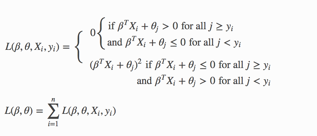
Again, you can add the Regularization Penalty to the loss function. The model parameters are adjusted by minimizing the loss function using gradient descent. When the Ordinal family is specified, the solver parameter will automatically be set to GRADIENT_DESCENT_LH and use the log-likelihood function. To adjust the model parameters using the loss function, you can set the solver parameter to GRADIENT_DESCENT_SQERR.

Because only first-order methods are used in adjusting the model parameters, use Grid Search to choose the best combination of the obj_reg, alpha, and lambda parameters.

In general, the loss function methods tend to generate better accuracies than the likelihood method. In addition, the loss function method is faster as it does not deal with logistic functions - just linear functions when adjusting the model parameters.

Pseudo-logistic regression (Quasibinomial family)

The quasibinomial family option works in the same way as the aforementioned binomial family. The difference is that binomial models only support 0/1 for the values of the target. A quasibinomial model supports "pseudo" logistic regression and allows for two arbitrary integer values (for example -4, 7). Additional information about the quasibinomial option can be found in the "Estimating Effects on Rare Outcomes: Knowledge is Power" paper.

Multiclass classification (Multinomial family)

Multinomial family generalization of the binomial model is used for multi-class response variables. Similar to the binomial family, GLM models the conditional probability of observing class c given x. A vector of coefficients exists for each of the output classes. ($\beta$ is a matrix.) The probabilities are defined as:

$\hat{y}_c = Pr(y = c|x) = \frac{e^{x^\top\beta_c + \beta_{c0}}}{\sum^K_{k=1}(e^{x^\top\beta_k+\beta_{k0}})}$

The penalized negative log-likelihood is defined as:

$- \Big[ \dfrac {1} {N} \sum_{i=1}^N \sum_{k=1}^K \big( y_{i,k} (x^T_i \beta_k + \beta_{k0}) \big) - \text{log} \big( \sum_{k=1}^K e^{x{^T_i}\beta_k + {\beta_{k0}}} \big) \Big] + \lambda \Big[ \dfrac {(1-\alpha)} {2} ||\beta || ^2_F + \alpha \sum_{j=1}^P ||\beta_j ||_1 \Big]$

where $\beta_c$ is a vector of coefficients for class c, and $y_{i,k}$ is the $k\text{th}$ element of the binary vector produced by expanding the response variable using one-hot encoding (that is, $y_{i,k} == 1$ iff the response at the $i\text{th}$ observation is k; otherwise it is 0.)

Poisson models

Poisson regression is typically used for datasets where the response represents counts, and the errors are assumed to have a Poisson distribution. In general, it can be applied to any data where the response is non-negative. It models the dependency between the response and covariates as:

$\hat {y} = e^{x{^T}\beta + {\beta_{0}}}$

The model is fitted by maximizing the corresponding penalized likelihood:

$^\text{max}_{\beta,\beta_0} \dfrac {1} {N} \sum_{i=1}^{N} \Big( y_i(x_{i}^{T}\beta + \beta_0) - e^{x{^T_i}\beta + {\beta_0}} \Big)- \lambda \Big( \alpha||\beta||_1 + \dfrac {1} {2}(1 - \alpha)||\beta||^2_2 \Big)$

The corresponding deviance is equal to:

$D = -2 \sum_{i=1}^{N} \big( y_i \text{log}(y_i / \hat {y}_i) - (y_i - \hat {y}_i) \big)$

Note in the equation above that H2O-3 Secure uses the negative log of the likelihood. This is different than the way deviance is specified in https://onlinecourses.science.psu.edu/stat501/node/377/. In order to use this deviance definition, simply multiply the H2O-3 Secure deviance by -1.

Gamma models

The gamma distribution is useful for modeling a positive continuous response variable, where the conditional variance of the response grows with its mean, but the coefficient of variation of the response $\sigma^2(y_i)/\mu_i$ is constant. It is usually used with the log link $g(\mu_i) = \text{log}(\mu_i)$ or the inverse link $g(\mu_i) = \dfrac {1} {\mu_i}$, which is equivalent to the canonical link.

The model is fitted by solving the following likelihood maximization:

$^\text{max}_{\beta,\beta_0} - \dfrac {1} {N} \sum_{i=1}^{N} \dfrac {y_i} {x{^T_i}\beta + \beta_0} + \text{log} \big( x{^T_i}\beta + \beta_0 \big ) - \lambda \Big( \alpha||\beta||_1 + \dfrac {1} {2}(1 - \alpha)||\beta||^2_2 \Big)$

The corresponding deviance is equal to:

$D = 2 \sum_{i=1}^{N} - \text{log} \bigg (\dfrac {y_i} {\hat {y}_i} \bigg) + \dfrac {(y_i - \hat{y}_i)} {\hat {y}_i}$

Tweedie models

Tweedie distributions are a family of distributions that include gamma, normal, Poisson, and their combinations. Tweedie distributions are especially useful for modeling positive continuous variables with exact zeros. The variance of the Tweedie distribution is proportional to the $p$-th power of the mean $var(y_i) = \phi\mu{^p_i}$, where $\phi$ is the dispersion parameter and $p$ is the variance power.

The Tweedie distribution is parametrized by variance power $p$ while $\phi$ is an unknown constant. It is defined for all $p$ values except in the (0,1) interval and has the following distributions as special cases:

• $p = 0$: Normal
• $p = 1$: Poisson
• $p \in (1,2)$: Compound Poisson, non-negative with mass at zero
• $p = 2$: Gamma
• $p = 3$: Inverse-Gaussian
• $p > 2$: Stable, with support on the positive reals

The model likelihood to maximize has the form:

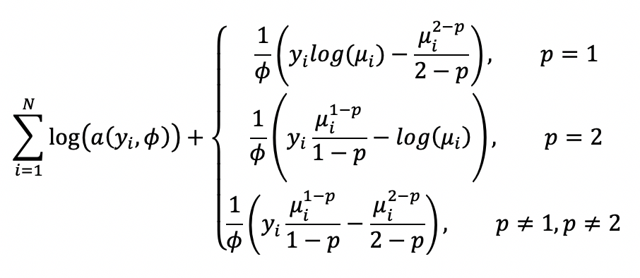
where the function $a(y_i,\phi)$ is evaluated using an infinite series expansion and does not have an analytical solution. However, because $\phi$ is an unknown constant, $\sum_{i=1}^N\text{log}(a(y_i,\phi))$ is a constant and will be ignored. Hence, the final objective function to minimize with the penalty term is:

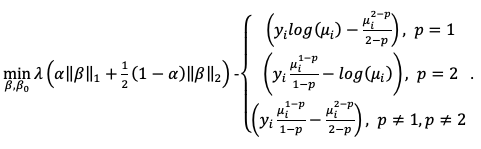
The link function in the GLM representation of the Tweedie distribution defaults to:

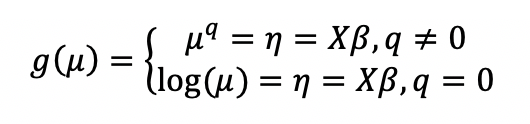
And $q = 1 - p$. The link power $q$ can be set to other values as well.

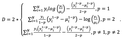
The corresponding deviance is equal to:

Negative Binomial models

Negative binomial regression is a generalization of Poisson regression that loosens the restrictive assumption that the variance is equal to the mean. Instead, the variance of negative binomial is a function of its mean and parameter $\theta$, the dispersion parameter.

Let $Y$ denote a random variable with negative binomial distribution, and let $\mu$ be the mean. The variance of $Y (\sigma^2)$ will be $\sigma^2 = \mu + \theta\mu^2$. The possible values of $Y$ are non-negative integers: 0, 1, 2, and so on.

The negative binomial regression for an observation $i$ is:

$Pr(Y = y_i|\mu_i, \theta) = \frac{\Gamma(y_i+\theta^{-1})}{\Gamma(\theta^{-1})\Gamma(y_i+1)} {\bigg(\frac {1} {1 + {\theta {\mu_i}}}\bigg) ^\theta}^{-1} { \bigg(\frac {{\theta {\mu_i}}} {1 + {\theta {\mu_i}}} \bigg) ^{y_i}}$

where $\Gamma(x)$ is the gamma function, and $\mu_i$ can be modeled as:

$$\begin{aligned} \mu_i=\left\{ \begin{array}{ll} exp (\beta^T X_i + \beta_0) \text{ for log link}\\ \beta^T X_i + \beta_0 \text{ for identity link}\\ \end{array} \right. \end{aligned}$$

The negative log likelihood $L(y_i,\mu_i)$ function is:

$^\text{max}_{\beta,\beta_0} \bigg[ \frac{-1}{N} \sum_{i=1}^{N} \bigg \{ \bigg( \sum_{j=0}^{y_i-1} \text{log}(j + \theta^{-1} ) \bigg) - \text{log} (\Gamma (y_i + 1)) - (y_i + \theta^{-1}) \text{log} (1 + \theta\mu_i) + y_i \text{log}(\mu_i) + y_i \text{log} (\theta) \bigg \} \bigg]$

The final penalized negative log likelihood is used to find the coefficients $\beta, \beta_0$ given a fixed $\theta$ value:

$L(y_i, \mu_i) + \lambda \big(\alpha || \beta || _1 + \frac{1}{2} (1 - \alpha) || \beta || _2 \big)$

The corresponding deviance is:

$D = 2 \sum_{i=1}^{N} \bigg \{ y_i \text{log} \big(\frac{y_i}{\mu_i} \big) - (y_i + \theta^{-1}) \text{log} \frac{(1+\theta y_i)}{(1+\theta \mu_i)} \bigg \}$

note

Future versions of this model will optimize the coefficients as well as the dispersion parameter.

Links

As indicated previously, a link function $g$: $E(y) = \mu = {g^-1}(\eta)$ relates the expected value of the response $\mu$ to the linear component $\eta$. The link function can be any monotonic differentiable function. This relaxes the constraints on the additivity of the covariates, and it allows the response to belong to a restricted range of values depending on the chosen transformation $g$.

H2O's GLM supports the following link functions: Family_Default, Identity, Logit, Log, Inverse, Tweedie, and Ologit.

The following table describes the allowed Family/Link combinations.

Family	Link Function
	Family_Default	Identity	Logit	Log	Inverse	Tweedie	Ologit
Binomial	X		X
Fractional Binomial	X		X
Quasibinomial	X		X
Multinomial	X
Ordinal	X						X
Gaussian	X	X		X	X
Poisson	X	X		X
Gamma	X	X		X	X
Tweedie	X					X
Negative Binomial	X	X		X
AUTO	X***	X*	X**	X*	X*

For AUTO:

• X*: the data is numeric (Real or Int) (family determined as gaussian)
• X**: the data is Enum with cardinality = 2 (family determined as binomial)
• X***: the data is Enum with cardinality > 2 (family determined as multinomial)

Dispersion parameter estimation

Regularization is not supported when you use dispersion parameter estimation with maximum likelihood.

Tweedie

The density for the maximum likelihood function for Tweedie can be written as:

$f( y; \theta, \phi) = a (y, \phi, p) \exp \Big[ \frac{1}{\phi} \big\{ y \theta - k(\theta) \big\} \Big] \quad \text{Equation 1}$

where:

• $a (y, \phi, p), k(\theta)$ are suitable known functions
• $\phi$ is the dispersion parameter and is positive
• $\theta = \begin{cases} \frac{\mu ^{1-p}}{1-p} & p \neq 1 \\ \log (\mu) & p = 1 \end{cases}$
• $k(\theta) = \begin{cases} \frac{\mu ^{2-p}}{2-p} & p \neq 2 \\ \log (\mu) & p=2 \end{cases}$
• the value of $\alpha (y,\phi)$ depends on the value of $p$

If there are weights introduced to each data row, equation 1 will become:

$f \Big( y; \theta, \frac{\phi}{w} \Big) = a \Big( y, \frac{\phi}{w}, p \Big) \exp \Big[ \frac{w}{\phi} \big\{ y\theta - k(\theta) \big\} \Big]$

$\alpha (y,\phi)$ when $1 < p < 2$

For $Y=0$,

$P(Y=0) = \exp \Big\{-\frac{\mu^{2-p}}{\phi (2-p)} \Big\} \quad \text{Equation 2}$

For $Y>0$,

$a(y, \phi, p) = \frac{1}{y} W(y, \phi, p) \quad \text{Equation 3}$

with $W(y, \phi, p) = \sum^{\infty}_{j=1} W_j$ and

$W_j = \frac{y^{-j \alpha}(p-1)^{\alpha j}}{\phi^{j(1-\alpha)} (2-p)^j j! \Gamma(-j\alpha)} \quad \text{Equation 4}$

If weight is applied to each row, equation 4 becomes:

$W_j = \frac{w^{j(1-\alpha)}y^{-j \alpha}(p-1)^{\alpha j}}{\phi^{j(1-\alpha)}(2-p)^j j! \Gamma(-j \alpha)} \quad \text{Equation 5}$

The $W_j$ terms are all positive. The following figure plots for $\mu = 0.5, p=1.5, \phi =1. y=0.1$.

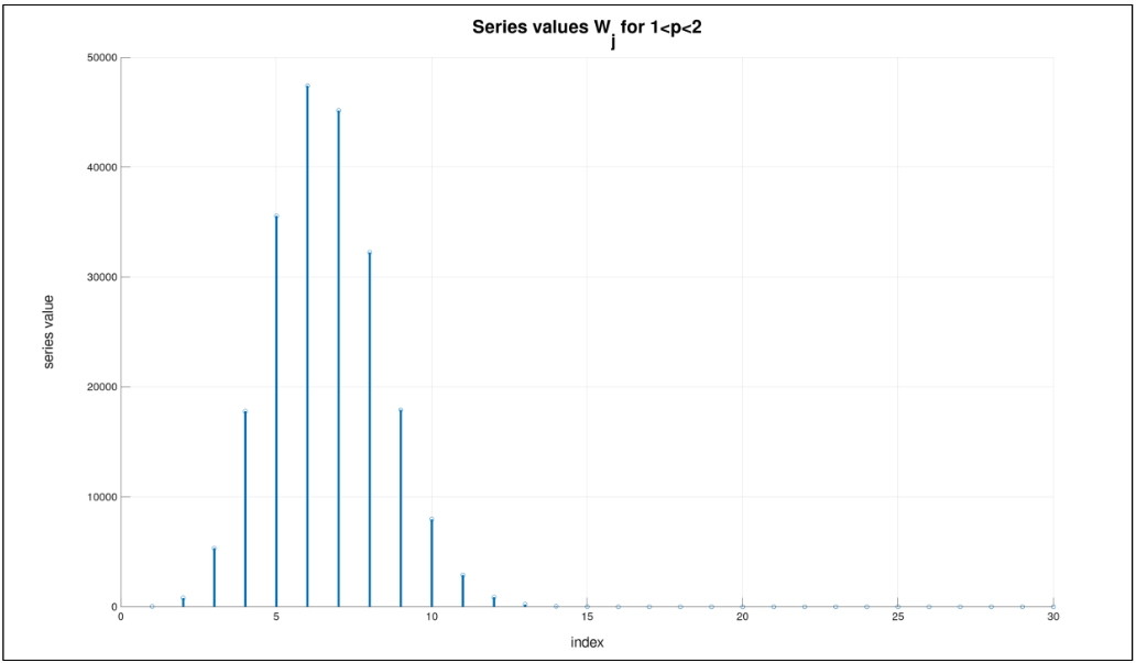
$\alpha (y,\phi)$ when $p > 2$

Here, you have

$a(y, \phi, p) = \frac{1}{\pi y}V(y,\phi, p) \quad \text{Equation 6}$

and $V = \sum^{\infty}_{k=1} V_k$ where

$V_k = \frac{\Gamma(1+\alpha k)\phi^{k(\alpha - 1)}(p-1)^{\alpha k}}{\Gamma(1+k)(p-2)^ky^{\alpha k}}(-1)^k \sin (-k\pi \alpha) \quad \text{Equation 7}$

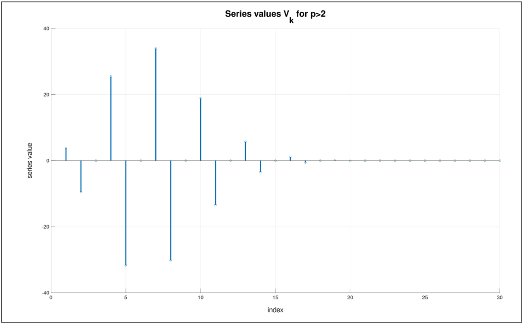
Note that $0 < \alpha < 1$ for $p>2$. The $V_k$ terms are both positive and negative. This will limit the numerical accuracy that is obtained in summing it as shown in the following image. Again, if weights are applied to each row of the dataset, equation 6 becomes:

$V_k = \frac{\Gamma(1+\alpha k)\phi^{k(\alpha -1)}(p-1)^{\alpha k}}{\Gamma(1+k)w^{k(\alpha -1)}(p-2)^ky^{\alpha k}}(-1)^k \sin (-k\pi \alpha) \quad \text{Equation 8}$

In the following figure, we use $\mu =0.5,p=2.5,\phi =1, y=0.1$.

Warnings

Accuracy and Limitation

While the Tweedie's probability density function contains an infinite series sum, when $p$ is close to 2, the response ($y$) is large, and $\phi$ is small the common number of terms that are needed to approximate the infinite sum grow without bound. This causes an increase in computation time without reaching the desired accuracy.

Multimodal Densities

As $p$ closes in on 1, the Tweedie density function becomes multimodal. This means that the optimization procedure will fail since it will not be able to find the global optimal point. It will instead arrive at a local optimal point.

As a conservative condition, to ensure that the density is unimodal for most values of $y,\phi$, we should have $p>1.2$.

Tweedie dispersion example

R

# Import the training data:
training_data <- h2o.importFile("http://h2o-public-test-data.s3.amazonaws.com/smalldata/glm_test/tweedie_p3_phi1_10KRows.csv")

# Set the predictors and response:
predictors <- c('abs.C1.', 'abs.C2.', 'abs.C3.', 'abs.C4.', 'abs.C5.')
response <- 'x'

# Build and train the model:
model <- h2o.glm(x = predictors, 
                 y = response, 
                 training_frame = training_data, 
                 family = 'tweedie',
                 tweedie_variance_power = 3, 
                 lambda = 0, 
                 compute_p_values = TRUE, 
                 dispersion_parameter_method = "pearson", 
                 init_dispersion_parameter = 0.5, 
                 dispersion_epsilon = 1e-4, 
                 max_iterations_dispersion = 100)

# Retrieve the estimated dispersion:
model@model$dispersion
[1] 0.7599965

Python

# Import the training data:
training_data = h2o.import_file("http://h2o-public-test-data.s3.amazonaws.com/smalldata/glm_test/tweedie_p3_phi1_10KRows.csv")

# Set the predictors and response:
predictors = ["abs.C1.", "abs.C2.", "abs.C3.", "abs.C4.", "abs.C5."]
response = "x"

# Build and train the model:
model = H2OGeneralizedLinearEstimator(family="tweedie", 
                                      lambda_=0, 
                                      compute_p_values=True, 
                                      dispersion_parameter_method="pearson", 
                                      init_dispersion_parameter=0.5, 
                                      dispersion_epsilon=1e-4,
                                      tweedie_variance_power=3, 
                                      max_iterations_dispersion=100)
model.train(x=predictors, y=response, training_frame=training_data)

# Retrieve the estimated dispersion:
model._model_json["output"]["dispersion"]
0.7599964835351135

Negative Binomial

GLM dispersion estimation using the maximum likelihood method for the negative binomial family is available when you set dispersion_parameter_method=“ml”.

The coefficients, or betas, are estimated using IRLSM. The dispersion parameter theta is estimated after each IRLSM iteration. After the first beta update, the initial theta estimate is made using the method of moments as a starting point. Then, theta is updated using the maximum likelihood in each iteration.

While not converged:

1. Estimate coefficients (betas)
2. Estimate dispersion (theta)
   1. If it is the first iteration:
      1. Theta $\gets$ Method of Moments estimate
   2. Otherwise:
      1. Theta $\gets$ Maximum Likelihood estimate using Newton’s method with learning rate estimated using Golden section search

Regularization

Regularization is used to attempt to solve problems with overfitting that can occur in GLM. Penalties can be introduced to the model building process to avoid overfitting, to reduce variance of the prediction error, and to handle correlated predictors. The two most common penalized models are ridge regression and LASSO (least absolute shrinkage and selection operator). The elastic net combines both penalties using both the alpha and lambda options (that is, values greater than 0 for both).

LASSO and ridge regression

LASSO represents the $\ell{_1}$ penalty and is an alternative regularized least squares method that penalizes the sum of the absolute coefficents $||\beta||{_1} = \sum{^p_{k=1}} \beta{^2_k}$. LASSO leads to a sparse solution when the tuning parameter is sufficiently large. As the tuning parameter value $\lambda$ is increased, all coefficients are set to zero. Because reducing parameters to zero removes them from the model, LASSO is a good selection tool.

Ridge regression penalizes the $\ell{_2}$ norm of the model coefficients $||\beta||{^2_2} = \sum{^p_{k=1}} \beta{^2_k}$. It provides greater numerical stability and is easier and faster to compute than LASSO. It keeps all the predictors in the model and shrinks them proportionally. Ridge regression reduces coefficient values simultaneously as the penalty is increased without setting any of them to zero.

Variable selection is important in numerous modern applications with many covariates where the $\ell{_1}$ penalty has proven to be successful. H2O recommends using LASSO if the number of variables is large or if the solution is known to be sparse, as it selects a small number of variables for sufficiently high $\lambda$—which can be important to the interpretability of the model. The $\ell{_2}$ norm does not have this effect; it shrinks the coefficients but does not set them exactly to zero.

The two penalties also differ in the presence of correlated predictors. The $\ell{_2}$ penalty shrinks coefficients for correlated columns toward each other, while the $\ell{_1}$ penalty tends to select only one of them and sets the other coefficients to zero. Using the elastic net argument $\alpha$ combines these two behaviors.

The elastic net method selects variables and preserves the grouping effect (shrinking coefficients of correlated columns together). Moreover, while the number of predictors that can enter a LASSO model saturates at min $(n,p)$ (where $n$ is the number of observations, and $p$ is the number of variables in the model), the elastic net does not have this limitation and can fit models with a larger number of predictors.

Elastic net penalty

As indicated previously, elastic net regularization is a combination of the $\ell{_1}$ and $\ell{_2}$ penalties parametrized by the $\alpha$ and $\lambda$ arguments (similar to "Regularization Paths for Generalized Linear Models via Coordinate Descent" by Friedman et al.).

• $\alpha$ controls the elastic net penalty distribution between the $\ell_1$ and $\ell_2$ norms. It can have any value in the [0,1] range or a vector of values (via grid search). If $\alpha=0$, then H2O solves the GLM using ridge regression. If $\alpha=1$, then LASSO penalty is used.
• $\lambda$ controls the penalty strength. The range is any positive value or a vector of values (via grid search). Note that $\lambda$ values are capped at $\lambda_{max}$, which is the smallest $\lambda$ for which the solution is all zeros (except for the intercept term).

The combination of the $\ell_1$ and $\ell_2$ penalties is beneficial because $\ell_1$ induces sparsity, while $\ell_2$ gives stability and encourages the grouping effect (where a group of correlated variables tend to be dropped or added into the model simultaneously). When focusing on sparsity, one possible use of the $\alpha$ argument involves using the $\ell_1$ mainly with minimal $\ell_2$ ($\alpha$ almost 1) to stabilize the computation and improve convergence speed.

Regularization parameters in GLM

To get the best possible model, find the optimal values of the regularization parameters $\alpha$ and $\lambda$. H2O supports a grid search over $\alpha$ and a special form of grid search called "lambda search" over $\lambda$.

The recommended way to find optimal regularization settings on H2O is to do a grid search over a few $\alpha$ values with an automatic lambda search for each $\alpha$.

• Alpha

  The alpha parameter controls the distribution between the $\ell{_1}$ (LASSO) and $\ell{_2}$ (ridge regression) penalties. A value of 1.0 for alpha represents LASSO, and an alpha value of 0.0 produces ridge regression.

• Lambda

  The lambda parameter controls the amount of regularization applied. If lambda is 0.0, no regularization is applied, and the alpha parameter is ignored. The default value for lambda is calculated by H2O using a heuristic based on the training data. If you allow H2O to calculate the value for lambda, you can see the chosen value in the model output.

Lambda search

If the lambda_search option is set, GLM will compute models for full regularization path similar to glmnet. (See the glmnet paper.) Regularization path starts at lambda max (highest lambda values which makes sense—that is, the lowest value driving all coefficients to zero) and goes down to lambda min on log scale, decreasing regularization strength at each step. The returned model will have coefficients corresponding to the “optimal” lambda value as decided during training.

When looking for a sparse solution (alpha > 0), lambda search can also be used to efficiently handle wide datasets because it can filter out inactive predictors (noise) and only build models for a small subset of predictors. A possible use case for lambda search is to run it on a dataset with many predictors but limit the number of active predictors to a relatively small value.

Lambda search can be configured along with the following arguments:

• alpha: Regularization distribution between $\ell_1$ and $\ell_2$.

• validation_frame and/or nfolds: Used to select the best lambda based on the cross-validation performance or the validation or training data. If available, cross-validation performance takes precedence. If no validation data is available, the best lambda is selected based on training data performance and is therefore guaranteed to always be the minimal lambda computed since GLM cannot overfit on a training dataset.

  note

  If running lambda search with a validation dataset and cross-validation disabled, the chosen lambda value corresponds to the lambda with the lowest validation error. The validation dataset is used to select the model, and the model performance should be evaluated on another independent test dataset.

• lambda_min_ratio and nlambdas: The sequence of the $\lambda$ values is automatically generated as an exponentially decreasing sequence. It ranges from $\lambda_{max}$ (the smallest $\lambda$ so that the solution is a model with all zeros) to $\lambda_{min} =$ lambda_min_ratio $\times$ $\lambda_{max}$.

  H2O computes $\lambda$ models sequentially and in decreasing order, warm-starting the model (using the previous solution as the initial prediction) for $\lambda_k$ with the solution for $\lambda_{k-1}$. By warm-starting the models, we get better performance. Typically models for subsequent $\lambda$ values are close to each other, so only a few iterations per $\lambda$ are needed (two or three). This also achieves greater numerical stability because models with a higher penalty are easier to compute. This method starts with an easy problem and then continues to make small adjustments.

  note

  lambda_min_ratio and nlambdas also specify the relative distance of any two lambdas in the sequence. This is important when applying recursive strong rules, which are only effective if the neighboring lambdas are "close" to each other. The default value for lambda_min_ratio is $1e^{-4}$, and the default value for nlambdas is 100. This gives a ratio of 0.912. For best results when using strong rules, keep the ratio close to this default.

• max_active_predictors: This limits the number of active predictors. (The actual number of non-zero predictors in the model is going to be slightly lower.) It is useful when obtaining a sparse solution to avoid costly computation of models with too many predictors.

Full regularization path

It can sometimes be useful to see the coefficients for all lambda values or to override default lambda selection. Full regularization path can be extracted from both the R and Python clients. It returns coefficients (and standardized coefficients) for all computed lambda values and also the explained deviances on both train and validation. Subsequently, the makeGLMModel call can be used to create an H2O GLM model with selected coefficients.

To extract the regularization path from R or python:

• R: call h2o.getGLMFullRegularizationPath. This takes the model as an argument. An example is available here.
• Python: H2OGeneralizedLinearEstimator.getGLMRegularizationPath (static method). This takes the model as an argument. An example is available here.

Solvers

This section provides general guidelines for best performance from the GLM implementation details. The optimal solver depends on the data properties and prior information regarding the variables (if available). In general, the data are considered sparse if the ratio of zeros to non-zeros in the input matrix is greater than 10. The solution is sparse when only a subset of the original set of variables is intended to be kept in the model. In a dense solution, all predictors have non-zero coefficients in the final model.

In GLM, you can specify one of the following solvers:

• IRLSM: Iteratively Reweighted Least Squares Method (default)
• L_BFGS: Limited-memory Broyden-Fletcher-Goldfarb-Shanno algorithm
• AUTO: Sets the solver based on given data and parameters.
• COORDINATE_DESCENT: Coordinate Decent (not available when family=multinomial)
• COORDINATE_DESCENT_NAIVE: Coordinate Decent Naive
• GRADIENT_DESCENT_LH: Gradient Descent Likelihood (available for Ordinal family only; default for Ordinal family)
• GRADIENT_DESCENT_SQERR: Gradient Descent Squared Error (available for Ordinal family only)

IRLSM and L-BFGS

IRLSM (the default) uses a Gram Matrix approach, which is efficient for tall and narrow datasets and when running lambda search via a sparse solution. For wider and dense datasets (thousands of predictors and up), the L-BFGS solver scales better. If there are fewer than 500 predictors (or so) in the data, use the default solver (IRLSM). For larger numbers of predictors, run IRLSM with a lambda search, then compare it to L-BFGS with just one $\ell_2$ penalty. The following general guidelines apply:

• For a dense solution and a dense dataset, use IRLSM if there are fewer than 500 predictors in the data; otherwise, use L-BFGS. Set alpha=0 to include $\ell_2$ regularization in the elastic net penalty term to avoid inducing sparsity in the model.
• For a dense solution with a sparse dataset, use IRLSM if there are fewer than 2000 predictors in the data; otherwise, use L-BFGS. Set alpha=0.
• For a sparse solution with a dense dataset, use IRLSM with lambda_search=TRUE if fewer than 500 active predictors in the solution are expected; otherwise, use L-BFGS. Set alpha to be greater than 0 to add in an $\ell_1$ penalty to the elastic net regularization, which induces sparsity in the estimated coefficients.
• For a sparse solution with a sparse dataset, use IRLSM with lambda_search=TRUE if you expect less than 5000 active predictors in the solution; otherwise, use L-BFGS. Set alpha to be greater than 0.

If you are unsure whether the solution should be sparse or dense, try both along with a grid of alpha values. The optimal model can be picked based on its performance on the validation data (or alternatively, based on the performance in cross-validation when not enough data is available to have a separate validation dataset).

Coordinate descent

In addition to IRLSM and L-BFGS, H2O's GLM includes options for specifying Coordinate Descent. Cyclical Coordinate Descent is able to handle large datasets well and deals efficiently with sparse features. It can improve the performance when the data contains categorical variables with a large number of levels, as it is implemented to deal with such variables in a parallelized way.

• Coordinate Descent is IRLSM with the covariance updates version of cyclical coordinate descent in the innermost loop. This version is faster when $N > p$ and $p$ ~ $500$.
• Coordinate Descent Naive is IRLSM with the naive updates version of cyclical coordinate descent in the innermost loop.
• Coordinate Descent provides much better results if lambda search is enabled. Also, with bounds, it tends to get higher accuracy.
• Coordinate Descent cannot be used with family=multinomial.

Both of the above method are explained in the glmnet paper.

Gradient descent

For Ordinal regression problems, H2O provides options for Gradient Descent. Gradient Descent is a first-order iterative optimization algorithm for finding the minimum of a function. In H2O's GLM, conventional ordinal regression uses a likelihood function to adjust the model parameters. The model parameters are adjusted by maximizing the log-likelihood function using gradient descent. When the Ordinal family is specified, the solver parameter will automatically be set to GRADIENT_DESCENT_LH. To adjust the model parameters using the loss function, you can set the solver parameter to GRADIENT_DESCENT_SQERR.

Coefficients table

A Coefficients Table is outputted in a GLM model. This table provides the following information: Column names, Coefficients, Standard Error, z-value, p-value, and Standardized Coefficients.

• Coefficients are the predictor weights (that is, the weights used in the actual model used for prediction) in a GLM model.
• Standard error, z-values, and p-values are classical statistical measures of model quality. p-values are essentially hypothesis tests on the values of each coefficient. A high p-value means that a coefficient is unreliable (insignificant) while a low p-value suggests that the coefficient is statistically significant.
• The standardized coefficients are returned if the standardize option is enabled (which is the default). These are the predictor weights of the standardized data and are included only for informational purposes (for example, to compare relative variable importance). In this case, the "normal" coefficients are obtained from the standardized coefficients by reversing the data standardization process (de-scaled, with the intercept adjusted by an added offset) so that they can be applied to data in its original form (that is, no standardization prior to scoring). Note: These are not the same as coefficients of a model built on non-standardized data.

Extracting coefficients table information

You can extract the columns in the Coefficients Table by specifying names, coefficients, std_error, z_value, p_value, standardized_coefficients in a retrieve/print statement. (Refer to the example that follows.) In addition, H2O provides the following built-in methods for retrieving standard and non-standard coefficients:

• coef(): Coefficients that can be applied to non-standardized data
• coef_norm(): Coefficients that can be fitted on the standardized data (requires standardized=TRUE, which is the default)

For an example, refer to the Examples section.

GLM likelihood

Maximum likelihood estimation

For an initial rough estimate of the parameters $\hat{\beta}$ you use the estimate to generate fitted values: $\mu_{i}=g^{-1}(\hat{\eta_{i}})$

Let $z$ be a working dependent variable such that $z_{i}=\hat{\eta_{i}}+(y_{i}-\hat{\mu_{i}})\frac{d\eta_{i}}{d\mu_{i}}$, where $\frac{d\eta_{i}}{d\mu_{i}}$ is the derivative of the link function evaluated at the trial estimate.

Calculate the iterative weights: $w_{i}=\frac{p_{i}}{[b^{\prime\prime}(\theta_{i})\frac{d\eta_{i}}{d\mu_{i}}^{2}]}$, where $b^{\prime\prime}$ is the second derivative of $b(\theta_{i})$ evaluated at the trial estimate.

Assume $a_{i}(\phi)$ is of the form $\frac{\phi}{p_{i}}$. The weight $w_{i}$ is inversely proportional to the variance of the working dependent variable $z_{i}$ for current parameter estimates and proportionality factor $\phi$.

Regress $z_{i}$ on the predictors $x_{i}$ using the weights $w_{i}$ to obtain new estimates of $\beta$:

$\hat{\beta}=(\mathbf{X}^{\prime}\mathbf{W}\mathbf{X})^{-1}\mathbf{X}^{\prime}\mathbf{W}\mathbf{z}$

where $\mathbf{X}$ is the model matrix, $\mathbf{W}$ is a diagonal matrix of $w_{i}$, and $\mathbf{z}$ is a vector of the working response variable $z_{i}$.

This process is repeated until the estimates $\hat{\beta}$ change by less than the specified amount.

Likelihood and AIC

During model training, simplified formulas of likelihood and AIC are used. After the model is built, the full formula is used to calculate the output of the full log likelihood and full AIC values. The full formula is used to calculate the output of the full log likelihood and full AIC values if the parameter calc_like is set to True.

note

The log likelihood value is not available in the cross-validation metrics. The AIC value is available and is calculated using the original simplified formula independent of the log likelihood.

The following are the supported GLM families and formulae (the log likelihood is calculated for the i th observation).

Gaussian:

$l(\mu_i (\beta); y_i, w_i) = - \frac{1}{2} \Big[ \frac{w_i (y_i - \mu_i)^2}{\phi} + \log \big(\frac{\phi}{w_i} \big) + \log (2 \pi) \Big]$

where

• $\phi$ is the dispersion parameter estimation
• $\mu_i$ is the prediction
• $y_i$ is the real value of the target variable

note

For Gaussian family, you need the dispersion parameter estimate in order to calculate the full log likelihood and AIC. Hence, when calc_like is set to True, the parameters compute_p_values and remove_collinear_columns are set to True. The parameter dispersion_parameter_method is set to "pearson" by default. However, you can set the dispersion_parameter_method to deviance if you prefer.

Binomial:

$l \big(\mu_i (\beta); y_i, w_i \big) = w_i \big(y_i \log \{ \mu_i \} + (1-y_i) \log \{ 1-\mu_i \} \big)$

where

• $\mu_i$ is the probability of 1
• $y_i$ is the real value of the target variable

Quasibinomial:

• If the predicted value equals $y_i$, log likelihood is 0

• If $\mu_i >1$ then $l(\mu_i (\beta); y_i) = y_i \log \{ \mu_i \}$

• Otherwise, $l(\mu_i (\beta); y_i) = y_i \log \{ \mu_i \} + (1-y_i) \log \{ 1- \mu_i \}$ where

  • $\mu_i$ is the probability of 1
  • $y_i$ is the real value of the target variable

Fractional Binomial:

$l(\mu_i (\beta); y_i) = w_i \Big(y_i \times \log \big(\frac{y_i}{\mu_i} \big) + (1-y_i) \times \log \big(\frac{1-y_i}{1-\mu_i} \big) \Big)$

where

• $\mu_i$ is the probability of 1
• $y_i$ is the real value of the target variable

Poisson:

$l(\mu_i (\beta); y_i) = w_i \big(y_i \times \log (\mu_i) - \mu_i - \log (\Gamma (y_i +1)) \big)$

where

• $\mu_i$ is the prediction
• $y_i$ is the real value of the target variable

Negative Binomial:

$l(\mu_i (\beta); y_i, w_i) = y_i \log \big(\frac{k \mu}{w_i} \big) - \big(y_i + \frac{w_i}{k} \big) \log \big(1 + \frac{k \mu}{w_i} \big) + \log \Big(\frac{\Gamma \big( y_i + \frac{w_i}{k} \big)} {\Gamma (y_i +1) \Gamma \big(\frac{w_i}{k}\big)} \Big)$

where

• $\mu_i$ is the prediction
• $y_i$ is the real value of the target variable
• $k = \frac{1}{\phi}$ is the dispersion parameter estimation

note

For Negative Binomial family, you need the dispersion parameter estimate. When the parameter calc_like is set to True, the parameters compute_p_values and remove_collinear_columns are set to True for you. By default, the parameter dispersion_parameter_method is set to "pearson". However, you can set dispersion_parameter_method to "deviance" or "ml" if you prefer.

Gamma:

$l(\mu_i (\beta); y_i, w_i) = \frac{w_i}{\phi} \log \big( \frac{w_i y_i}{\phi \mu_i} \big) - \frac{w_i y_i}{\phi \mu_i} - \log (y_i) - \log \big(\Gamma \big(\frac{w_i}{\phi} \big) \big)$

where

• $\mu_i$ is the prediction
• $y_i$ is the real value of the target variable
• $\phi$ is the dispersion parameter estimation

note

For Gamma family, you need the dispersion parameter estimate. When the parameter calc_like is set to True, the parameters compute_p_values and remove_collinear_columns are set to True for you. By default, the parameter dispersion_parameter_method is set to "pearson". However, you can set dispersion_parameter_method to "deviance" or "ml" if you prefer.

Multinomial:

$l(\mu_i(\beta); y_i) = w_i \log (\mu_i)$

where $\mu_i$ is the predicted probability of the actual class $y_i$

Tweedie:

The Tweedie calculation is located in the section Tweedie Likelihood Calculation.

note

For Tweedie family, you need the dispersion parameter estimate. When the parameter calc_like is set to True, the dispersion_parameter_method is set to "ml" which provides you with the best log likelihood estimation.

Final AIC calculation

The final AIC in the output metric is calculated using the standard formula, utilizing the previously computed log likelihood.

$\text{AIC} = -2LL + 2p$

where

• $p$ is the number of estimated coefficients (that is, including dispersion etc). When using regularization $p$ is the number of non-zero coefficients.
• $LL$ is the log likelihood

To manage computational intensity, calc_like is used. This parameter was previously only used for HGLM models, but its utilization has been expanded. By default, calc_like=False, but you can set it to True and the parameter HGLM to False to enable the calculation of the full log likelihood and full AIC. This computation is performed during the final scoring phase after the model finishes building.

note

For ridge regression and elastic net, the AIC is approximated without calculating the actual effective degrees of freedom—that is, the estimate is the same as for LASSO. Therefore, the AIC values for ridge regression and elastic net should be used with caution.

Tweedie likelihood calculation

Three estimations are used to calculate Tweedie likelihood:

• when you fix the variance power and estimate the dispersion parameter;
• when you fix the dispersion parameter and estimate the variance power; or
• when you estimate both the variance power and dispersion parameter.

The calculation in this section is used to estimate the full log likelihood. When you fix the Tweedie variance power, you will use a simpler formula (unless you are estimating dispersion). When fixing the Tweedie variance power for dispersion estimation, you use the Series method.

When you fix the variance power and estimate the dispersion parameter, the Series method is used to perform the estimation. In this case, you can actually separate the GLM coefficient estimation and the dispersion parameter estimation at the end of the GLM model building process. Standard Newton's method is used to estimate the dispersion parameter using the Series method which is an approximation of the Tweedie likelihood function.

Depending on $p$, $y$, and $\phi$, different methods are used for this log likelihood estimation. To start, let:

$\xi = \frac{\phi}{y^{2-p}}$

If $p=2$, then it will use the log likelihood of the Gamma distribution:

$$\begin{aligned} \log (p) = \begin{cases} - \infty & y=0 \\ \frac{1}{\phi} \log (\frac{1}{\phi \mu}) - \log \text{Gamma} \frac{1}{\phi} + \log (y)(\frac{1}{\phi} -1) + (-\frac{1}{\phi \mu} y) & y>0 \end{cases} \end{aligned}$$

If $p=3$, then it will use the inverse Gaussian distribution:

$$\begin{aligned} \log (p) = \begin{cases} - \infty & y=0 \\ \frac{1}{2} \Big( -\log (\phi \mu) - \log (2 \pi) - 3 \log \big( \frac{y}{\mu} \big) - \frac{(\frac{y}{\mu} -1)^2}{\phi \mu \frac{y}{\mu}} \Big) - \log (\mu) & y>0 \end{cases} \end{aligned}$$

If $p<2$ and $\xi \leq 0.01$, then it will use the Fourier inversion method.

If $p>2$ and $\xi \geq 1$, then it will also use the Fourier inversion method.

Everything else will use the Series method. However, if the Series method fails (output of NaN), then it will try the Fourier inversion method instead.

If both the Series method and Fourier inversion method fail, or if the Fourier inversion method was chosen based on the $\xi$ criterium and it failed, it will then estimate the log likelihood using the Saddlepoint approximation.

Here are the general usages for Tweedie variance power and dispersion parameter estimation using maximum likelihood:

• fix_tweedie_variance_power = True and fix_dispersion_parameter = False as it will use the Tweedie variance power set in parameter tweedie_variance_power and estimate the dispersion parameter starting with the value set in parameter init_dispersion_parameter;
• fix_tweedie_variance_power = False and fix_dispersion_parameter = True as it will use the dispersion parameter value in parameter init_dispersion_parameter and estimate the Tweedie variance power starting with the value set in parameter tweedie_variance_power;
• fix_tweedie_variance_power = False and fix_dispersion_parameter = False as it will estimate both the variance power and dispersion parameter using the values set in tweedie_variance_power and init_dispersion_parameter respectively.

Optimization Procedure

When estimating just the Tweedie variance power, it uses the golden section search. Once a small region is found, then it switches to Newton's method. If Newton's method fails (that is, steps out of the bounds found by the golden section search), it uses the golden section search until convergence. When you optimize both Tweedie variance power and dispersion, it uses the Nelder-Mead method with constraints so that Tweedie variance power $p>1+10^{-10}$ and dispersion $\phi >10^{-10}$. If the Nelder-Mead seems to be stuck in local optimum, you might want to try increasing the dispersion_learning_rate.

note

(Applicable for Gamma, Tweedie, and Negative Binomial families) If you set dispersion_parameter_method="ml", then solver must be set to "IRLSM".

Variable inflation factors

The variable inflation factor (VIF) quantifies the inflation of the variable. Variables are inflated due to their correlation with other predictor variables within the model. For each predictor in a multiple regression model, there is a VIF. This process can be calculated with cross validation turned on.

The VIF is constructed by:

• setting a numerical predictor x as the response while using the remaining predictors except for y,
• building a GLM regression model,
• calculating the VIF as $\frac{1.0}{(1.0-R^2)}$ where $R^2$ is taken from the GLM regression model built in the prior step, and
• repeating this process for all remaining numerical predictors to retrieve their VIF.

Variable inflation factor example

R

# Import the training data:
training_data <- h2o.importFile("http://h2o-public-test-data.s3.amazonaws.com/smalldata/glm_test/gamma_dispersion_factor_9_10kRows.csv")

# Set the predictors and response:
predictors <- c('abs.C1.','abs.C2.','abs.C3.','abs.C4.','abs.C5.')
response <- 'resp'

# Build and train the model:
vif_glm <- h2o.glm(x = predictors, 
                   y = response, 
                   training_frame = training_data, 
                   family = 'gamma', 
                   lambda = 0, 
                   generate_variable_inflation_factors = TRUE, 
                   fold_assignment = 'modulo', 
                   nfolds = 3, 
                   keep_cross_validation_models = TRUE)

# Retrieve the variable inflation factors:
h2o.get_variable_inflation_factors(vif_glm)
 abs.C1.  abs.C2.  abs.C3.  abs.C4.  abs.C5. 
1.000334 1.000173 1.000785 1.000539 1.000535 

Python

# Import the GLM estimator:
from h2o.estimators import H2OGeneralizedLinearEstimator

# Import the training data:
training_data = h2o.import_file("http://h2o-public-test-data.s3.amazonaws.com/smalldata/glm_test/gamma_dispersion_factor_9_10kRows.csv")

# Set the predictors and response:
predictors = ["abs.C1.","abs.C2.","abs.C3.","abs.C4.","abs.C5."]
response = "resp"

# Build and train the model:
vif_glm = H2OGeneralizedLinearEstimator(family="gamma", 
                                        lambda_=0, 
                                        generate_variable_inflation_factors=True, 
                                        fold_assignment="modulo", 
                                        nfolds=3, 
                                        keep_cross_validation_models=True)
vif_glm.train(x=predictors, y=response, training_frame=training_data)

# Retrieve the variable inflation factors:
vif_glm.get_variable_inflation_factors()
{'Intercept': nan, 'abs.C1.': 1.0003341467438167, 'abs.C2.': 1.0001734204183244, 'abs.C3.': 1.0007846189027745, 'abs.C4.': 1.0005388379729434, 'abs.C5.': 1.0005349427184604}

Constrained GLM

The algorithm is based on Bierlaire's Optimization: Principles and Algorithms, Chapter 19 [8] where we're basically trying to solve the following optimization problem:

$\min_{X\in R^n} f(x), \text{subject to } h(x) = 0, g(x) \leq 0 \quad \text{ equation 1}$

where:

• $f: R^n \to R,h: R^n \to R^m,g: R^n \to R^p$
• the constraints $h,g$ are linear.

However, the actual problem we are solving is:

$\min_{X\in R^n} f(x) \text{ subject to } h(x)=0 \quad \text{ equation 2}$

The inequalities constraints can be easily converted to equalities constraints through simple reasoning and using active constraints. We solve the constrained optimization problem by solving the augmented Lagrangian function using the quadratic penalty:

$L_c(x,\lambda) = f(x) + \lambda^T h(x) + \frac{c}{2} \| h(x) \|^2 \quad \text{ equation 3}$

The basic ideas used to solve the constrained GLM consist of:

1. transforming a constrained problem into a sequence of unconstrained problems;
2. penalizing more and more the possible violation of the constraints during the sequence by continuously increasing the value of $c$ at each iteration.

Converting to standard form

A standard form of $g(x) \leq 0$ is the only acceptable form of inequality constraints. For example, if you have a constraint of $2x_1 - 4x_2 \geq 10$ where $x_1 \text{ and } x_4$ are coefficient names, then you must convert it to $10-2x_1 + 4x_2 \leq 0$.

Example of constrained GLM

R

# Import the Gaussian 10,000 rows dataset:
h2o_data <- h2o.importFile("https://s3.amazonaws.com/h2o-public-test-data/smalldata/glm_test/gaussian_20cols_10000Rows.csv")

# Set the predictors, response, and enum columns:
enum_columns = c("C1", "C2", "C3", "C4", "C5", "C6", "C7", "C8", "C9", "C10")
for (cname in enum_columns) {
h2o.asfactor(h2o_data[cname])
}
myY = "C21"
col_names <- names(h2o_data)
myX <- col_names[1:20]

# Set the constraints:
constraints <- data.frame(names <- c("C1.2", "C11", "constant", "C5.2", "C12", "C15", "constant"),
values <- c(1, 1, 13.56, 1, 1, 1, -5),
types <- c("Equal", "Equal", "Equal", "LessThanEqual", "LessThanEqual", "LessThanEqual", "LessThanEqual"),
constraint_numbers <- c(0, 0, 0, 1, 1, 1, 1))
constraints_h2o <- as.h2o(constraints)

# Set the beta constraints:
bc <- data.frame(names <- c("C1.1", "C5.2", "C11", "C15"), 
                 lower_bounds <- c(-36, -14, 25, 14), 
                 upper_bounds <- c(-35, -13, 26, 15))
bc_h2o <- as.h2o(bc)

# Build and train your model:
m_sep <- h2o.glm(x=myX, 
                 y=myY, 
                 training_frame=h2o_data, 
                 family='gaussian', 
                 linear_constraints=constraints_h2o, 
                 solver="irlsm", 
                 lambda=0.0, 
                 beta_constraints=bc_h2o, 
                 constraint_eta0=0.1, 
                 constraint_tau=10, 
                 constraint_alpha=0.01, 
                 constraint_beta=0.9, 
                 constraint_c0=100)

# Find your coefficients:
h2o.coef(m_sep)

Python

# Import the Gaussian 10,000 rows dataset:
h2o_data = h2o.import_file("https://s3.amazonaws.com/h2o-public-test-data/smalldata/glm_test/gaussian_20cols_10000Rows.csv")

# Set the predictors, response, and enum columns:
enum_columns = ["C1", "C2", "C3", "C4", "C5", "C6", "C7", "C8", "C9", "C10"]
for cname in enum_columns:
    h2o_data[cname] = h2o_data[cname].asfactor()
myY = "C21"
myX = h2o_data.names.remove(myY)

# Set the linear constraints:
linear_constraints = [] # this constraint is satisfied by default coefficient initialization
name = "C1.2"
values = 1
types = "Equal"
contraint_numbers = 0
linear_constraints.append([name, values, types, contraint_numbers])

name = "C11"
values = 1
types = "Equal"
contraint_numbers = 0
linear_constraints.append([name, values, types, contraint_numbers])

name = "constant"
values = 13.56 
types = "Equal"
contraint_numbers = 0
linear_constraints.append([name, values, types, contraint_numbers])

name = "C5.2"
values = 1
types = "LessThanEqual"
contraint_numbers = 1
linear_constraints.append([name, values, types, contraint_numbers])

name = "C12"
values = 1
types = "LessThanEqual"
contraint_numbers = 1
linear_constraints.append([name, values, types, contraint_numbers])

name = "C15"
values = 1
types = "LessThanEqual"
contraint_numbers = 1
linear_constraints.append([name, values, types, contraint_numbers])

name = "constant"
values = -5
types = "LessThanEqual"
contraint_numbers = 1
linear_constraints.append([name, values, types, contraint_numbers])

linear_constraints2 = h2o.H2OFrame(linear_constraints)
linear_constraints2.set_names(["names", "values", "types", "constraint_numbers"])

# Set the beta constraints:
bc = []
name = "C1.1"
c1p1LowerBound = -36
c1p1UpperBound=-35
bc.append([name, c1p1LowerBound, c1p1UpperBound])

name = "C5.2"
c5p2LowerBound=-14
c5p2UpperBound=-13
bc.append([name, c5p2LowerBound, c5p2UpperBound])

name = "C11"
c11LowerBound=25
c11UpperBound=26
bc.append([name, c11LowerBound, c11UpperBound])

name = "C15"
c15LowerBound=14
c15UpperBound=15
bc.append([name, c15LowerBound, c15UpperBound])

beta_constraints = h2o.H2OFrame(bc)
beta_constraints.set_names(["names", "lower_bounds", "upper_bounds"])

# Build and train your model:
m_sep = glm(family='gaussian', 
            linear_constraints=linear_constraints2, 
            solver="irlsm", 
            lambda_=0.0, 
            beta_constraints=beta_constraints, 
            constraint_eta0=0.1, 
            constraint_tau=10, 
            constraint_alpha=0.01, 
            constraint_beta=0.9, 
            constraint_c0=100)
m_sep.train(training_frame=h2o_data,x=myX, y=myY)

# Find your coefficients:
coef_sep = m_sep.coef()

Treatment of strict inequalities

To convert a strict inequality, just add a small number to it. For example, $2x_1 - 4x_2 < 0$ can be converted to $2x_1 - 4x_2 - 10^{-12} \leq 0$.

Transforming inequality constraints to equality constraints

This transformation is going to use slack variables which are introduced to replace an inequality constraint by an equality constraint. The slack variable should be non-negative. To transform inequality constraints to equality constraints, we proceed as follows:

1. For each inequality constraint of $g(x)$, a slack variable is added to it such that you will have: $g_i(x) - s_i^2 = 0$;
2. Let $s = \begin{bmatrix} s_1^2 \\ \vdots \\ s_p^2 \end{bmatrix}$ and $g_{aug}(x) = g(x) - s$;
3. When $g_i(x) \leq 0$, the constraint is satisfied and can therefore be ignored and declared inactive;
4. The inequality constraints are violated only when $g_i(x) - s_i^2 \geq 0$. This is because it implies that $g_i(x) \geq s_i^2 \geq 0$ and this isn't allowed. Therefore, $geq(x)$ only includes the $g_i(x)$ when you have $g_i(x) \geq 0$;
5. Therefore, you have $h_a(x) = \begin{bmatrix} h(x) \\ geq(x) \end{bmatrix}$, where $h(x)$ is the original equality constraint and $geq(x)$ contains the inequality constraints that satisfied the condition $g_i(x) \geq 0$;
6. The optimization problem in equation 1 can now be rewritten as:

$\min_{X\in R^n} f(x), \text{ subject to } h_a(x) = 0 \quad \text{ equation 4}$

7. The augmented Lagrangian function you will solve from equation 4 becomes:

$L_c(x, \lambda) = f(x) + \lambda^T h_a(x) + \frac{c}{2} \|h_a(x)\|^2 \quad \text{ equation 5}$

Modifying or creating a custom GLM model

In R and Python, the makeGLMModel call can be used to create an H2O model from given coefficients. It needs a source GLM model trained on the same dataset to extract the dataset information. To make a custom GLM model from R or Python:

• R: call h2o.makeGLMModel. This takes a model, a vector of coefficients, and (optional) decision threshold as parameters.
• Python: H2OGeneralizedLinearEstimator.makeGLMModel (static method) takes a model, a dictionary containing coefficients, and (optional) decision threshold as parameters.

Examples

This code demonstrates how to build a Generalized Linear Model (GLM) using H2O-3 Secure with a binomial family for binary classification. The model is trained on the prostate dataset and computes p-values, standardized coefficients, and generates a scoring history. Additionally, it shows how to obtain the coefficients and the standardized coefficients, evaluates model performance, and retrieves model attributes like the number of active predictors.

R

library(h2o)
h2o.init()

df <- h2o.importFile("https://h2o-public-test-data.s3.amazonaws.com/smalldata/prostate/prostate.csv")
df$CAPSULE <- as.factor(df$CAPSULE)
df$RACE <- as.factor(df$RACE)
df$DCAPS <- as.factor(df$DCAPS)
df$DPROS <- as.factor(df$DPROS)

predictors <- c("AGE", "RACE", "VOL", "GLEASON")
response <- "CAPSULE"

prostate_glm <- h2o.glm(family = "binomial", 
                        x = predictors, 
                        y = response, 
                        training_frame = df, 
                        lambda = 0, 
                        compute_p_values = TRUE,
                        generate_scoring_history = TRUE)

# Coefficients that can be applied to the non-standardized data
h2o.coef(prostate_glm)
  Intercept      RACE.1      RACE.2         AGE         VOL     GLEASON 
-6.67515539 -0.44278752 -0.58992326 -0.01788870 -0.01278335  1.25035939

# Coefficients fitted on the standardized data (requires standardize=TRUE, which is on by default)
h2o.coef_norm(prostate_glm)
  Intercept      RACE.1      RACE.2         AGE         VOL     GLEASON 
-0.07610006 -0.44278752 -0.58992326 -0.11676080 -0.23454402  1.36533415 

# Print the coefficients table
prostate_glm@model$coefficients_table
Coefficients: glm coefficients
      names coefficients std_error   z_value  p_value standardized_coefficients
1 Intercept    -6.675155  1.931760 -3.455478 0.000549                 -0.076100
2    RACE.1    -0.442788  1.324231 -0.334373 0.738098                 -0.442788
3    RACE.2    -0.589923  1.373466 -0.429514 0.667549                 -0.589923
4       AGE    -0.017889  0.018702 -0.956516 0.338812                 -0.116761
5       VOL    -0.012783  0.007514 -1.701191 0.088907                 -0.234544
6   GLEASON     1.250359  0.156156  8.007103 0.000000                  1.365334

# Print the standard error
prostate_glm@model$coefficients_table$std_error
[1] 1.931760363 1.324230832 1.373465793 0.018701933 0.007514354 0.156156271

# Print the p values
prostate_glm@model$coefficients_table$p_value
[1] 5.493181e-04 7.380978e-01 6.675490e-01 3.388116e-01 8.890718e-02
[6] 1.221245e-15

# Print the z values
prostate_glm@model$coefficients_table$z_value
[1] -3.4554780 -0.3343734 -0.4295143 -0.9565159 -1.7011907  8.0071033

# Retrieve a graphical plot of the standardized coefficient magnitudes
h2o.std_coef_plot(prostate_glm)

# Since you generated the scoring history, you can retrieve the average objective and the negative log likelihood:
print(h2o.average_objective(prostate_glm))
[1] 0.540688
print(h2o.negative_log_likelihood(prostate_glm))
[1] 205.4614

Python

import h2o
h2o.init()
from h2o.estimators.glm import H2OGeneralizedLinearEstimator

prostate = h2o.import_file("https://h2o-public-test-data.s3.amazonaws.com/smalldata/prostate/prostate.csv")
prostate['CAPSULE'] = prostate['CAPSULE'].asfactor()
prostate['RACE'] = prostate['RACE'].asfactor()
prostate['DCAPS'] = prostate['DCAPS'].asfactor()
prostate['DPROS'] = prostate['DPROS'].asfactor()

predictors = ["AGE", "RACE", "VOL", "GLEASON"]
response_col = "CAPSULE"

prostate_glm = H2OGeneralizedLinearEstimator(family= "binomial", 
                                          lambda_ = 0, 
                                          compute_p_values = True,
                                          generate_scoring_history = True)
prostate_glm.train(predictors, response_col, training_frame= prostate)

# Coefficients that can be applied to the non-standardized data.
print(prostate_glm.coef())
{u'GLEASON': 1.2503593867263176, u'VOL': -0.012783348665664449, u'AGE': -0.017888697161812357, u'Intercept': -6.6751553940827195, u'RACE.2': -0.5899232636956354, u'RACE.1': -0.44278751680880707}

# Coefficients fitted on the standardized data (requires standardize = True, which is on by default)
print(prostate_glm.coef_norm())
{u'GLEASON': 1.365334151581163, u'VOL': -0.2345440232267344, u'AGE': -0.11676080128780757, u'Intercept': -0.07610006436753876, u'RACE.2': -0.5899232636956354, u'RACE.1': -0.44278751680880707}

# Print the Coefficients table
prostate_glm._model_json['output']['coefficients_table']
Coefficients: glm coefficients
names      coefficients    std_error    z_value    p_value      standardized_coefficients
---------  --------------  -----------  ---------  -----------  ---------------------------
Intercept  -6.67516        1.93176      -3.45548   0.000549318  -0.0761001
RACE.1     -0.442788       1.32423      -0.334373  0.738098     -0.442788
RACE.2     -0.589923       1.37347      -0.429514  0.667549     -0.589923
AGE        -0.0178887      0.0187019    -0.956516  0.338812     -0.116761
VOL        -0.0127833      0.00751435   -1.70119   0.0889072    -0.234544
GLEASON    1.25036         0.156156     8.0071     1.22125e-15  1.36533

# Print the Standard error
print(prostate_glm._model_json['output']['coefficients_table']['std_error'])
[1.9317603626604352, 1.3242308316851008, 1.3734657932878116, 0.01870193337051072, 0.007514353657915356, 0.15615627100850296]

# Print the p values
print(prostate_glm._model_json['output']['coefficients_table']['p_value'])
[0.0005493180609459358, 0.73809783692024, 0.6675489550762566, 0.33881164088847204, 0.0889071809658667, 1.2212453270876722e-15]

# Print the z values
print(prostate_glm._model_json['output']['coefficients_table']['z_value'])
[-3.4554779791058787, -0.3343733631736653, -0.42951434726559384, -0.9565159284557886, -1.7011907141473064, 8.007103260414265]

# Retrieve a graphical plot of the standardized coefficient magnitudes
prostate_glm.std_coef_plot()

# Since you generated the scoring history, you can access the average objective and negative log likelihood:
print("average objective: {0}.".format(prostate_glm.average_objective()))
average objective: 0.5406879877388551.
print("negative log likelihood: {0}.".format(prostate_glm.negative_log_likelihood()))
negative log likelihood: 205.46143534076492.

Calling model attributes

While not all model attributes have their own callable APIs, you can still retrieve their information. Using the previous example, here is how to call a model's attributes:

R

# Retrieve all model attributes:
prostate_glm@model$model_summary
GLM Model: summary
    family  link regularization number_of_predictors_total
1 binomial logit           None                          5
  number_of_active_predictors number_of_iterations  training_frame
1                           5                    4 RTMP_sid_8b2d_6

# Retrieve a specific model attribute (for example, the number of active predictors):
prostate_glm@model$model_summary['number_of_active_predictors']
number_of_active_predictors
1                         5

Python

# Retrieve all model attributes:
prostate_glm._model_json["output"]['model_summary']
GLM Model: summary
    family    link    regularization    number_of_predictors_total    number_of_active_predictors    number_of_iterations    training_frame
--  --------  ------  ----------------  ----------------------------  -----------------------------  ----------------------  ----------------
    binomial  logit   None              5                             5                              4                       py_4_sid_9981

# Retrieve a specific model attribute (for example, the number of active predictors):
prostate_glm._model_json["output"]['model_summary']['number_of_active_predictors']
['5']

FAQ

• How does the algorithm handle missing values during training?

  Depending on the selected missing value handling policy, they are either imputed mean or the whole row is skipped. The default behavior is Mean Imputation. Note that unseen categorical levels are replaced by the most frequent level present in training (mod). Optionally, GLM can skip all rows with any missing values.

• How does the algorithm handle missing values during testing?

  Same as during training. If the missing value handling is set to Skip and we are generating predictions, skipped rows will have Na (missing) prediction.

• What happens if the response has missing values?

  The rows with missing responses are ignored during model training and validation.

• What happens during prediction if the new sample has categorical levels not seen in training?

  The value will be filled with either 0 or replaced by the most frequent level present in training (if missing_value_handling was set to MeanImputation).

• How are unseen categorical values treated during scoring?

  Unseen categorical levels are treated based on the missing values handling during training. If your missing value handling was set to Mean Imputation, the unseen levels are replaced by the most frequent level present in training (mod). If your missing value treatment was Skip, the variable is ignored for the given observation.

• Does it matter if the data is sorted?

  No.

• Should data be shuffled before training?

  No.

• How does the algorithm handle highly imbalanced data in a response column?

  GLM does not require special handling for imbalanced data.

• What if there are a large number of columns?

  IRLS will get quadratically slower with the number of columns. Try L-BFGS for datasets with more than 5-10 thousand columns.

• What if there are a large number of categorical factor levels?

  GLM internally one-hot encodes the categorical factor levels; the same limitations as with a high column count will apply.

• When building the model, does GLM use all features or a selection of the best features?

  Typically, GLM picks the best predictors, especially if lasso is used (alpha = 1). By default, the GLM model includes an L1 penalty and will pick only the most predictive predictors.

• When running GLM, is it better to create a cluster that uses many smaller nodes or fewer larger nodes?

  A rough heuristic would be:

  $nodes \approx M \times N^2/(p \times 1e8)$

  where $M$ is the number of observations, $N$ is the number of columns (categorical columns count as a single column in this case), and $p$ is the number of CPU cores per node.

  For example, a dataset with 250 columns and 1M rows would optimally use about 20 nodes with 32 cores each (following the formula $250^2 \times 1000000/(32 \times 1e8) = 19.5 \approx 20$).

• How is variable importance calculated for GLM?

  For GLM, the variable importance represents the coefficient magnitudes.

• How does GLM define and check for convergence during logistic regression?

  GLM includes three convergence criteria outside of max iterations:

  • beta_epsilon: beta stops changing. This is used mostly with IRLSM.
  • gradient_epsilon: gradient is too small. This is used mostly with L-BFGS.
  • objective_epsilon: relative objective improvement is too small. This is used by all solvers.

  The default values below are based on a heuristic:

  • The default for beta_epsilon is 1e-4.
  • The default for gradient_epsilon is 1e-6 if there is no regularization (lambda = 0) or you are running with lambda_search; 1e-4 otherwise.
  • The default for objective_epsilon is 1e-6 if lambda = 0; 1e-4 otherwise.

  The default for max_iterations depends on the solver type and whether you run with lambda search:

  • for IRLSM, the default is 50 if no lambda search; 10* number of lambdas otherwise
  • for LBFGS, the default is number of classes (1 if not classification) * max(20, number of predictors /4 ) if no lambda search; it is number of classes * 100 * n-lambdas with lambda search.

  You will receive a warning if you reach the maximum number of iterations. In some cases, GLM can end prematurely if it can not progress forward via line search. This typically happens when running a lambda search with IRLSM solver. Note that using CoordinateDescent solver fixes the issue.

• Why do I receive different results when I run R’s glm and H2O’s glm?

  H2O’s glm and R’s glm do not run the same way and, thus, will provide different results. This is mainly due to the fact that H2O’s glm uses H2O math, H2O objects, and H2O distributed computing. H2O’s glm by default adds regularization, so it is essentially solving a different problem.

• How can I get H2O’s GLM to match R’s glm() function?

  To match R’s GLM, set the following in H2O’s GLM:

  solver = "IRLSM"
  lambda = 0
  remove_collinear_columns = TRUE
  compute_p_values = TRUE

  note

  beta_constraints must not be set.

GLM algorithm

Following the definitive text by P. McCullagh and J.A. Nelder (1989) on the generalization of linear models to non-linear distributions of the response variable Y, H2O fits GLM models based on the maximum likelihood estimation via iteratively reweighed least squares.

Let $y_{1},\dots,y_{n}$ be n observations of the independent, random response variable $Y_{i}$.

Assume that the observations are distributed according to a function from the exponential family and have a probability density function of the form:

$f(y_{i})=exp[\frac{y_{i}\theta_{i} - b(\theta_{i})}{a_{i}(\phi)} + c(y_{i}; \phi)]$ where $\theta$ and $\phi$ are location and scale parameters, and $a_{i}(\phi)$, $b_{i}(\theta{i})$, and $c_{i}(y_{i}; \phi)$ are known functions.

$a_{i}$ is of the form $a_{i}= \frac{\phi}{p_{i}}$ where $p_{i}$ is a known prior weight.

When $Y$ has a pdf from the exponential family:

$E(Y_{i})=\mu_{i}=b^{\prime} var(Y_{i})=\sigma_{i}^2=b^{\prime\prime}(\theta_{i})a_{i}(\phi)$

Let $g(\mu_{i})=\eta_{i}$ be a monotonic, differentiable transformation of the expected value of $y_{i}$. The function $\eta_{i}$ is the link function and follows a linear model.

$g(\mu_{i})=\eta_{i}=\mathbf{x_{i}^{\prime}}\beta$

When inverted: $\mu=g^{-1}(\mathbf{x_{i}^{\prime}}\beta)$

Cost of computation

H2O can process large data sets because it relies on parallel processes. Large data sets are divided into smaller data sets and processed simultaneously and the results are communicated between computers as needed throughout the process.

In GLM, data are split by rows but not by columns, because the predicted Y values depend on information in each of the predictor variable vectors. If O is a complexity function, N is the number of observations (or rows), and P is the number of predictors (or columns) then

$Runtime \propto p^3+\frac{(N*p^2)}{CPUs}$

Distribution reduces the time it takes an algorithm to process because it decreases N.

Relative to P, the larger that (N/CPUs) becomes, the more trivial p becomes to the overall computational cost. However, when p is greater than (N/CPUs), O is dominated by p.

  $Complexity = O(p^3 + N*p^2)$

References

Breslow, N E. “Generalized Linear Models: Checking Assumptions and Strengthening Conclusions.” Statistica Applicata 8 (1996): 23-41.

Peter K. Dunn, Gordon K. Symth, “Series evaluation of Tweedie exponential dispersion model densities”, Statistics and Computing, Volume 15 (2005), pages 267-280.

Jerome Friedman, Trevor Hastie, and Rob Tibshirani. Regularization Paths for Generalized Linear Models via Coordinate Descent. Journal of Statistical Software, 33(1), 2009.

Frome, E L. “The Analysis of Rates Using Poisson Regression Models.” Biometrics (1983): 665-674.

Goldberger, Arthur S. “Best Linear Unbiased Prediction in the Generalized Linear Regression Model.” Journal of the American Statistical Association 57.298 (1962): 369-375.

Guisan, Antoine, Thomas C Edwards Jr, and Trevor Hastie. “Generalized Linear and Generalized Additive Models in Studies of Species Distributions: Setting the Scene.” Ecological modeling 157.2 (2002): 89-100.

Nelder, John A, and Robert WM Wedderburn. “Generalized Linear Models.” Journal of the Royal Statistical Society. Series A (General) (1972): 370-384.

Lee, Y and Nelder, J. A. Hierarchical generalized linear models with discussion. J. R. Statist. Soc. B, 58:619-678, 1996.

Lee, Y and Nelder, J. A. and Y. Pawitan. Generalized linear models with random effects. Chapman & Hall/CRC, 2006.

Pearce, Jennie, and Simon Ferrier. “Evaluating the Predictive Performance of Habitat Models Developed Using Logistic Regression.” Ecological modeling 133.3 (2000): 225-245.

Press, S James, and Sandra Wilson. “Choosing Between Logistic Regression and Discriminant Analysis.” Journal of the American Statistical Association 73.364 (April, 2012): 699–705.

Snee, Ronald D. “Validation of Regression Models: Methods and Examples.” Technometrics 19.4 (1977): 415-428.

Ronnegard, Lars. HGLM course at the Roslin Institute, http://users.du.se/~lrn/DUweb/Roslin/RoslinCourse_hglmAlgorithm_Nov13.pdf.

Balzer, Laura B, and van der Laan, Mark J. "Estimating Effects on Rare Outcomes: Knowledge is Power." U.C. Berkeley Division of Biostatistics Working Paper Series (2013).

Michel Bierlaire, Optimization: Principles and Algorithms, Chapter 19, EPEL Press, second edition, 2018

---

Feedback

• Submit and view feedback for this page
• Send feedback about H2O-3 Secure to cloud-feedback@h2o.ai