H2O-3 Blogs
This page houses the most recent major release blog and focused content blogs for H2O.
Major Release Blogs
H2O Release 3.46

We are excited to announce the release of H2O-3 3.46.0.1! Some of the highlights of this major release are that we added custom metric support for XGBoost, allowed grid search models to be sorted with custom metrics, and we enabled H2O MOJO and POJO to work with MLFlow. Several improvements were also made to the Uplift model (like MLI support). Another exciting update is that we now allow GLM models that were previously built to be used to calculate full loglikelihood and AIC. We also focused on fixing security vulnerabilities. Please read on for more details!
Security patch updates
H2O should always be deployed behind firewalls and in protected clusters. Many of the reported vulnerabilities assume that H2O isn’t deployed under any protection. Regardless, there are several vulnerabilities we did fix during this release:
CVE-2023-6016: We introduced a Java Property that disables POJO import (defaults to
disabled) to avoid remote code execution (courtesy of Marek Novotný).CVE-2023-35116: We upgraded the jackson-databind version to address potential vulnerabilities (thanks to Marek Novotný).
SYNK-JAVA-CIMNUMBUSDS-6247633: We upgraded the nimbus-jose-jwt version to enhance security and to mitigate potential risks (kudos to Adam Valenta).
CVE-2023-6038 and CVE-2023-6569: We introduced a new configuration option for filtering file system access during reading and writing in response to security concerns (credit to Bartosz Krasinski).
XGBoost support for customized metrics (Adam Valenta)
XGBoost now supports the custom_metric_func parameter which lets you specify any desired metric. The custom_metric_func parameter is well known from other algorithms like GBM and Deep Learning. To see it in action, please look to our documentation.
Loglikelihood and AIC calculation support for GLM MOJOs (Yuliia Syzon)
GLM MOJOs now support the calculation of loglikelihood and AIC given a dataset with the response column when the MOJO is loaded with the H2O Generic model. To enable this feature, you have to build the GLM model with calc_like=True.
MLFlow Support (Marek Novotný)
We added the libraries from MLFlow (and necessary code) to enable you to use H2O-3 MOJO and POJO with the MLFlow frameworks.
Uplift DRF improvements (Veronika Maurerova)
In this release, we added many improvements for the Uplift DRF algorithm to provide you with more opportunities for tuning and interpreting your models. We added grid search, early stopping, partial dependence plots, and variable importance.
Python documentation improvements (Shaun Yogeshwaran)
We improved the Python documentation for the GAM, Model Selection, and ANOVA GLM algorithms by expanding the number of available examples. More will follow in the coming releases!
General Blogs
A Look at the UniformRobust method for histogram_type
Tree-based algorithms, especially Gradient Boosting Machines (GBM’s), are one of the most popular algorithms used. They often out-perform linear models and neural networks for tabular data since they used a boosted approach where each tree built works to fix the error of the previous tree. As the model trains, it is continuously self-correcting.
H2O-3’s GBM is able to train on real-world data out of the box: categoricals and missing values are automatically handled by the algorithm in a fully-distributed way. This means you can train the model on all your data without having to worry about sampling.
In this post, we talk about an improvement to how our GBM handles numeric columns. Traditionally, a GBM model would split numeric columns using uniform range-based splitting. Suppose you had a column that had values ranging from 0 to 100. It would split the column into bins 0-10, 11-20, 21-30, … 91-100. Each bin would be evaluated to determine the best way to split the data. The best split would be the one that most successfully splits your target column. For example, if you are trying to predict whether or not an employee will quit, the best split would be the one that could separate churn vs not-churn employees the most successfully.
However, when you’re handling data that has a column with outliers, this isn’t the most effective way to handle your data. Suppose you’re analyzing yearly income for a neighborhood: the vast majority of the people you’re looking at are making somewhere between $20-$80k. However, there are a few outliers in the neighborhood who make well-over $1 million. When splitting the column up for binning, it will still make uniform splits regardless of the distribution of data. Because the column splitting gets skewed with large outliers, all the outlier observations are classified into a single bin while the rest of the observations end up in another single bin. This, unfortunately, leaves most of the bins unused.
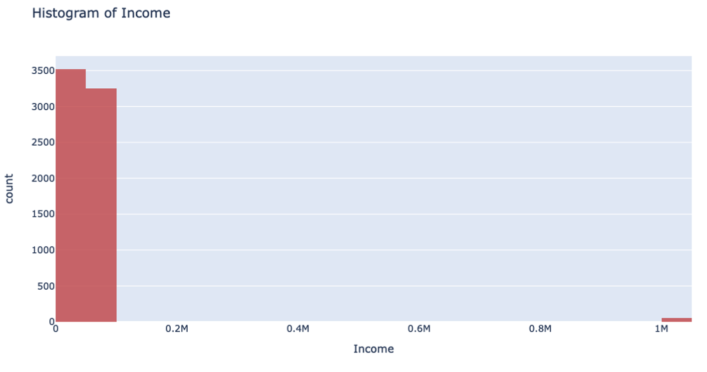
This can also drastically slow your prediction calculation since you’re iterating through so many empty bins. You also sacrifice accuracy because your data loses its diversity in this uneven binning method. Uniform splitting on data with outliers is full of issues.
The introduction of the UniformRobust method for histogram (histogram_type="UniformRobust") mitigates these issues! By learning from histograms from the previous layer, we are able to fine-tune the split points for the current layer.
The UniformRobust method isn’t impeded by outliers. It starts out using uniform range based binning. Then, it checks the distribution of the data in each bin. Many empty bins will indicate this range based binning is suboptimal, so it will iterate through all the bins and redefine them. If a bin contains no data, it’s deleted. If a bin contains too much data, then it’s split uniformly.
So, in the case that UniformRobust splitting fails (i.e. the distribution of values is still significantly skewed), the next iteration of finding splits attempts to correct the issue by repeating the procedure with new bins. This allows us to refine the promising bins recursively as we get deeper into the tree.
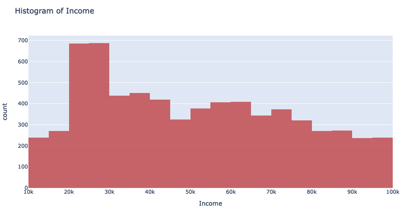
Let’s return to that income example. Using the UniformRobust method, we still begin with uniform splitting and see that very uneven distribution. However, what this method does next is to eliminate all those empty bins and split all the bins containing too much data. So, that bin that contained all the $0-100k yearly incomes is uniformly split. Then, with each iteration and each subsequent split, we will begin to see a much more even distribution of the data.
This method of splitting has the best available runtime performance and accuracy on datasets with outliers. We’re looking forward to you trying it out!
Example
In the following example, you can compare the performance of the UniformRobust method against the UniformAdaptive method on the Swedish motor insurance dataset. This dataset has slightly larger outliers in its Claims column.
library(h2o)
h2o.init()

# Import the Swedish motor insurance dataset. This dataset has larger outlier
# values in the "Claims" column:
motor <- h2o.importFile("http://h2o-public-test-data.s3.amazonaws.com/smalldata/glm_test/Motor_insurance_sweden.txt")

# Set the predictors and response:
predictors <- c("Payment", "Insured", "Kilometres", "Zone", "Bonus", "Make")
response <- "Claims"

# Build and train the UniformRobust model:
motor_robust <- h2o.gbm(histogram_type = "UniformRobust", seed = 1234, x = predictors, y = response, training_frame = motor)

# Build and train the UniformAdaptive model (we will use this model to
# compare with the UniformRobust model):
motor_adaptive <- h2o.gbm(histogram_type = "UniformAdaptive", seed = 1234, x = predictors, y = response, training_frame = motor)

# Compare the RMSE of the two models to see which model performed better:
print(c(h2o.rmse(motor_robust), h2o.rmse(motor_adaptive)))
[1] 36.03102 36.69582

# The RMSE is slightly lower in the UniformRobust model, showing that it performed better
# that UniformAdaptive on a dataset with outlier values!
import h2o
from h2o.estimators import H2OGradientBoostingEstimator
h2o.init()

# Import the Swedish motor insurance dataset. This dataset has larger outlier
# values in the "Claims" column:
motor = h2o.import_file("http://h2o-public-test-data.s3.amazonaws.com/smalldata/glm_test/Motor_insurance_sweden.txt")

# Set the predictors and response:
predictors = ["Payment", "Insured", "Kilometres", "Zone", "Bonus", "Make"]
response = "Claims"

# Build and train the UniformRobust model:
motor_robust = H2OGradientBoostingEstimator(histogram_type="UniformRobust", seed=1234)
motor_robust.train(x=predictors, y=response, training_frame=motor)

# Build and train the UniformAdaptive model (we will use this model to
# compare with the UniformRobust model):
motor_adaptive = H2OGradientBoostingEstimator(histogram_type="UniformAdaptive", seed=1234)
motor_adaptive.train(x=predictors, y=response, training_frame=motor)

# Compare the RMSE of the two models to see which model performed better:
print(motor_robust.rmse(), motor_adaptive.rmse())
36.03102136406947 36.69581743660738

# The RMSE is slightly lower in the UniformRobust model, showing that it performed better
# that UniformAdaptive on a dataset with outlier values!