Distributed Uplift Random Forest (Uplift DRF)
Introduction
Distributed Uplift Random Forest (Uplift DRF) is a classification tool for modeling uplift - the incremental impact of a treatment. Only binomial classification (distribution="bernoulli") is currently supported.
Uplift DRF can be applied in fields where we operate with two groups of subjects. First group, let’s call it treatment, receive some kind of treatment (e.g. marketing campaign, medicine,…), and a second group, let’s call it control, is separated from the treatment. We also gather information about their response, whether they bought a product, recover from disease, or similar. Then, Uplift DRF trains so-called uplift trees. Uplift trees take information about treatment/control group assignment and information about response directly into a decision about splitting a node. The output of the uplift model is the probability of change in user behavior which helps to decide if treatment impacts the desired behavior (e.g. buy a product, recover from disease,…). In other words, if a user responds because the user was treated. This leads to proper campaign targeting on a subject that genuinely needs to be treated and avoids wasting resources on subjects that respond/do not respond anyway.
The current version of Uplift DRF is based on the implementation of DRF because the principle of training is similar to DRF. When given a set of data, Uplift DRF generates a forest of classification uplift trees, rather than a single classification tree. Each of these trees is a weak learner built on a subset of rows and columns. More trees will reduce the variance. Classification take the average prediction over all of their trees to make a final prediction. (Note: For a categorical response column, Uplift DRF maps factors (e.g. ‘dog’, ‘cat’, ‘mouse) in lexicographic order to a name lookup array with integer indices (e.g. ‘cat -> 0, ‘dog’ -> 1, ‘mouse’ -> 2.)
Uplift DRF demo
Here is a Jupyter notebook where H2O Uplift DRF is compared to implementation Uplift RF from CausalML library.
Uplift metric
In Uplift Tree-based algorithms, every tree takes information about treatment/control group assignment and information about response directly into the decision about splitting a node. This means there is only one tree for both groups instead of separate trees for the treatment group’s data and the control group’s data.
Uplift DRF differentiates itself from DRF because it finds the best split using both response_column and treatment_column. The goal is to split the training observations into a group which gets an offer (i.e. treatment group) and a group which does not (i.e. control group). This information (treatment_column) with features and response_column are used for training. The uplift_metric is calculated to decide which point from the histogram is selected to split the data in the tree node (instead of calculation squared error or Gini coefficient like in other tree algorithms).
The goal is to maximize the differences between the class distributions in the treatment and control sets, so the splitting criteria are based on distribution divergences. The distribution divergence is calculated based on the uplift_metric parameter. In H2O-3, three uplift_metric types are supported:
Kullback-Leibler divergence (
uplift_metric="KL") - uses logarithms to calculate divergence, asymmetric, widely used, tends to infinity values (if treatment or control group distributions contain zero values). \(KL(P, Q) = \sum_{i=0}^{N} p_i \log{\frac{p_i}{q_i}}\)Squared Euclidean distance (
uplift_metric="euclidean") - symmetric and stable distribution, does not tend to infinity values. \(E(P, Q) = \sum_{i=0}^{N} (p_i-q_i)^2\)Chi-squared divergence (
uplift_metric="chi_squared") - Euclidean divergence normalized by control group distribution. Asymmetric and also tends to infinity values (if control group distribution contains zero values). \(X^2(P, Q) = \sum_{i=0}^{N} \frac{(p_i-q_i)^2}{q_i}\)
where:
\(P\) is treatment group distribution
\(Q\) is control group distribution
In a tree node the result value for a split is sum \(metric(P, Q) + metric(1-P, 1-Q)\). For the split gain value, the result within the node is normalized using the Gini coefficient (Euclidean or ChiSquared) or entropy (KL) for each distribution before and after the split.
You can read more information about uplift_metric on parameter specification page: uplift_metric.
Uplift tree and prediction
The uplift score is used as prediction of the leaf. Every leaf in a tree holds two predictions that are calculated based on a distribution of response between treatment and control group observations:
\(TP_l = (TY1_l + 1) / (T_l + 2)\)
\(CP_l = (CY1_l + 1) / (C_l + 2)\)
where:
\(l\) leaf of a tree
\(T_l\) how many observations in a leaf are from the treatment group (how many data rows in a leaf have
treatment_columnlabel == 1)\(C_l\) how many observations in a leaf are from the control group (how many data rows in the leaf have
treatment_columnlabel == 0)\(TY1_l\) how many observations in a leaf are from the treatment group and respond to the offer (how many data rows in the leaf have
treatment_columnlabel == 1 andresponse_columnlabel == 1)\(CY1_l\) how many observations in a leaf are from the control group and respond to the offer (how many data rows in the leaf have
treatment_columnlabel == 0 andresponse_columnlabel == 1)\(TP_l\) treatment prediction of a leaf
\(CP_l\) control prediction of a leaf
The uplift score for the leaf is calculated as the difference between the treatment prediction and the control prediction:
A higher uplift score means more observations from the treatment group responded to the offer than from the control group. This means the offered treatment has a positive effect. The uplift score can also be negative if more observations from the control group respond to the offer without treatment.
The final prediction is calculated in the same way as the DRF algorithm. Predictions for each observation are collected from all trees from an ensemble and the mean prediction is returned.
When the predict method is called on the test data, the result frame has these columns:
uplift_predict: result uplift prediction score, which is calculated asp_y1_with_treatment - p_y1_without_treatmentp_y1_with_treatment: probability the response is 1 if the row is from the treatment groupp_y1_without_treatment: probability the response is 1 if the row is from the control group
Extremely Randomized Trees
The same goes for Uplift DRF as does for random forests: a random subset of candidate features is used to determine the most discriminative thresholds that are picked as the splitting rule. In extremely randomized trees (XRT), randomness goes one step further in the way that splits are computed. As in random forests, a random subset of candidate features is used, but instead of looking for the most discriminative thresholds, thresholds are drawn at random for each candidate feature, and the best of these randomly generated thresholds is picked as the splitting rule. This usually allows to reduce the variance of the model a bit more, at the expense of a slightly greater increase in bias.
H2O supports extremely randomized trees (XRT) via histogram_type="Random". When this is specified, the algorithm will sample N-1 points from min…max and use the sorted list of those to find the best split. The cut points are random rather than uniform. For example, to generate 4 bins for some feature ranging from 0-100, 3 random numbers would be generated in this range (13.2, 89.12, 45.0). The sorted list of these random numbers forms the histogram bin boundaries e.g. (0-13.2, 13.2-45.0, 45.0-89.12, 89.12-100).
Defining an Uplift DRF Model
Parameters are optional unless specified as required.
Algorithm-specific parameters
auuc_nbins: Specify number of bins in a histogram to calculate Area Under Uplift Curve (AUUC). This option defaults to
-1which means 1000.auuc_type: The type of metric to calculate incremental uplift and then Area Under Uplift Curve (AUUC). Specify one of the following AUUC types:
autoorAUTO(default): Allow the algorithm to decide; Uplift DRF defaults toqiniqiniorQiniliftorLiftgainorGain
treatment_column: Specify the column which contains information about group dividing. The data must be categorical and have two categories:
0means the observation is in the control group and1means the observation is in the treatment group.uplift_metric: The type of divergence distribution to select the best split. Specify one of the following metrics:
autoorAUTO(default): Allow the algorithm to decide. In Uplift DRF, the algorithm will automatically performKLmetric.klorKL: Uses logarithms to calculate divergence (asymmetric, widely used, tends to infinity values if treatment or control group distributions contain zero values).euclideanorEuclidean: Symmetric and stable distribution (does not tend to infinity values).chi_squaredorChiSquared: Euclidean divergence normalized by control group distribution (asymmetric, tends to infinity values if control group distribution contains zero values).
Common parameters
categorical_encoding: Specify one of the following encoding schemes for handling categorical features:
autoorAUTO(default): Allow the algorithm to decide. In Uplift DRF, the algorithm will automatically performenumencoding.enumorEnum: 1 column per categorical feature.enum_limitedorEnumLimited: Automatically reduce categorical levels to the most prevalent ones during training and only keep the T (10) most frequent levels.one_hot_explicitorOneHotExplicit: N+1 new columns for categorical features with N levels.binaryorBinary: No more than 32 columns per categorical feature.eigenorEigen: k columns per categorical feature, keeping projections of one-hot-encoded matrix onto k-dim eigen space only.label_encoderorLabelEncoder: Convert every enum into the integer of its index (for example, level 0 -> 0, level 1 -> 1, etc.).sort_by_responseorSortByResponse: Reorders the levels by the mean response (for example, the level with lowest response -> 0, the level with second-lowest response -> 1, etc.). This is useful in GBM/DRF, for example, when you have more levels thannbins_cats, and where the top level splits now have a chance at separating the data with a split. Note that this requires a specified response column.
distribution: Specify the distribution (i.e., the loss function). The options are:
AUTO(default)bernoulli– response column must be 2-class categorical
ignore_const_cols: Specify whether to ignore constant training columns since no information can be gained from them. This option defaults to
True(enabled).ignored_columns: (Python and Flow only) Specify the column or columns to be excluded from the model. In Flow, click the checkbox next to a column name to add it to the list of columns excluded from the model. To add all columns, click the All button. To remove a column from the list of ignored columns, click the X next to the column name. To remove all columns from the list of ignored columns, click the None button. To search for a specific column, type the column name in the Search field above the column list. To only show columns with a specific percentage of missing values, specify the percentage in the Only show columns with more than 0% missing values field. To change the selections for the hidden columns, use the Select Visible or Deselect Visible buttons.
max_runtime_secs: Maximum allowed runtime in seconds for model training. Use
0(default) to disable.model_id: Specify a custom name for the model to use as a reference. By default, H2O automatically generates a destination key.
score_each_iteration: Enable this option to score during each iteration of the model training. This option defaults to
False(disabled).seed: Specify the random number generator (RNG) seed for algorithm components dependent on randomization. The seed is consistent for each H2O instance so that you can create models with the same starting conditions in alternative configurations. This option defaults to
-1(time-based random number).stopping_metric: Specify the metric to use for early stopping. The available options are:
AUTO(This defaults tologlossfor classification anddeviancefor regression)AUUC(area under the uplift curve, for UpliftDRF only)qini(difference between the Qini AUUC and area under the random uplift curve, for UpliftDRF only)ATE(average treatment effect, for UpliftDRF only)ATT(average treatment effect on the Treated, for UpliftDRF only)ATC(average treatment effect on the Control, for UpliftDRF only)
stopping_rounds: Stops training when the option selected for
stopping_metricdoesn’t improve for the specified number of training rounds, based on a simple moving average. To disable this feature, specify0(default). The metric is computed on the validation data (if provided); otherwise, training data is used.stopping_tolerance: Specify the relative tolerance for the metric-based stopping to stop training if the improvement is less than this value. This option defaults to
0.001.training_frame: Required Specify the dataset used to build the model.
NOTE: In Flow, if you click the Build a model button from the
Parsecell, the training frame is entered automatically.validation_frame: Specify the dataset used to evaluate the accuracy of the model.
verbose: Print scoring history to the console (metrics per tree). This option defaults to
False.x: Specify a vector containing the names or indices of the predictor variables to use when building the model. If
xis missing, then all columns exceptyare used.y: Required Specify the column to use as the dependent variable. The data must be categorical (only binomial classification is currently supported).
Leaf Node Assignment
Leaf Node assignment is not currently supported.
Interpreting an Uplift DRF Model
By default, the following output displays:
Model parameters (hidden)
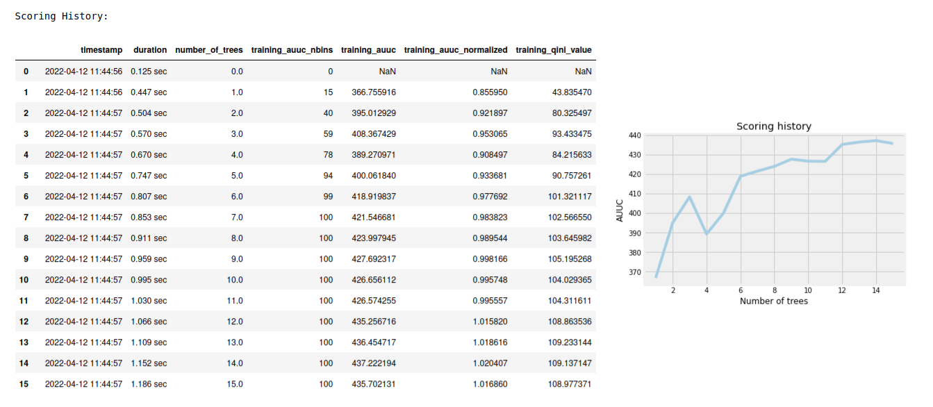
A graph of the scoring history (number of trees vs. training AUUC)
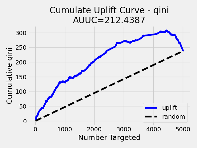
A graph of the AUUC curve (Number of observations vs. Uplift)
Output (model category, validation metrics)
Model summary (number of trees, min. depth, max. depth, mean depth, min. leaves, max. leaves, mean leaves)
Scoring history in tabular format
Training metrics (model name, checksum name, frame name, frame checksum name, description, model category, duration in ms, scoring time, predictions, ATE, ATT, ATC, AUUC, all AUUC types table, Thresholds and metric scores table)
Validation metrics (model name, checksum name, frame name, frame checksum name, description, model category, duration in ms, scoring time, predictions, ATE, ATT, ATC, AUUC, all AUUC types table, Thresholds and metric scores table)
Default AUUC metric calculated based on
auuc_typeparameterDefault normalized AUUC metric calculated based on
auuc_typeparameterAUUC table which contains all computed AUUC types and normalized AUUC (qini, lift, gain)
Qini value Average excess cumulative uplift (AECU) for qini metric type
AECU table which contains all computed AECU values types (qini, lift, gain)
Thresholds and metric scores table which contains thresholds of predictions, cumulative number of observations for each bin and cumulative uplift values for all metrics (qini, lift, gain).
Uplift Curve plot for given metric type (qini, lift, gain)
Variable Importance calculated based on Uplift Gain Improvement
Treatment effect metrics (ATE, ATT, ATC)
Overall treatment effect metrics show how the uplift predictions look across the whole dataset (population). Scored data are used to calculate these metrics (uplift_predict column = individual treatment effect).
Average Treatment Effect (ATE) Average expected uplift prediction (treatment effect) overall records in the dataset.
Average Treatment Effect on the Treated (ATT) Average expected uplift prediction (treatment effect) of all records in the dataset belonging to the treatment group.
Average Treatment Effect on the Control (ATC) Average expected uplift prediction (treatment effect) of all records in the dataset belonging to the control group.
The interpretation depends on concrete data meanings. We currently support only Bernoulli data distribution, so whether the treatment impacts the target value y=1 or not.
For example, we want to analyze data to determine if some medical will help to recover from a disease or not. We have patients in the treatment group and the control group. The target variable is if the medicine (treatment) helped recovery (y=1) or not (y=0). In this case: - positive ATE means the medicine helps with recovery in general - negative ATE means the medicine does not help with recovery in general - ATE equal to or close to zero means the medicine does not affect recovery in general - similar interpretation applies to ATT and ATC, the positive ATT is usually what scientists look for, but ATC is also an interesting metric (in an ideal case, positive both ATT and ATC say the treatment has an exact effect).
Custom metric example for Uplift DRF
import h2o
from h2o.estimators import H2OUpliftRandomForestEstimator
h2o.init()

# Import the cars dataset into H2O:
data = h2o.import_file("https://s3.amazonaws.com/h2o-public-test-data/smalldata/uplift/criteo_uplift_13k.csv")

# Set the predictors, response, and treatment column:
predictors = ["f1", "f2", "f3", "f4", "f5", "f6","f7", "f8"]
# set the response as a factor
response = "conversion"
data[response] = data[response].asfactor()
# set the treatment as a factor
treatment_column = "treatment"
data[treatment_column] = data[treatment_column].asfactor()

# Split the dataset into a train and valid set:
train, valid = data.split_frame(ratios=[.8], seed=1234)

# Define custom metric function
# ``pred`` is prediction array of length 3, where:
#   - pred[0]  = ``uplift_predict``: result uplift prediction score, which is calculated as ``p_y1_ct1 - p_y1_ct0``
#   - pred[1] = ``p_y1_ct1``: probability the response is 1 if the row is from the treatment group
#   - pred[2] = ``p_y1_ct0``: probability the response is 1 if the row is from the control group
# ``act`` is array with original data where
#   - act[0] = target variable
#   - act[1] = if the record belongs to the treatment or control group
# ``w`` (weight) and ``o`` (offset) are nor supported in Uplift DRF yet

class CustomAteFunc:
    def map(self, pred, act, w, o, model):
        return [pred[0], 1]

    def reduce(self, l, r):
        return [l[0] + r[0], l[1] + r[1]]

    def metric(self, l):
        return l[0] / l[1]

custom_metric = h2o.upload_custom_metric(CustomAteFunc, func_name="ate", func_file="mm_ate.py")

# Build and train the model:
uplift_model = H2OUpliftRandomForestEstimator(ntrees=10,
                                              max_depth=5,
                                              treatment_column=treatment_column,
                                              uplift_metric="KL",
                                              min_rows=10,
                                              seed=1234,
                                              auuc_type="qini"
                                              custom_metric_func=custom_metric)
uplift_model.train(x=predictors,
                   y=response,
                   training_frame=train,
                   validation_frame=valid)

# Eval performance:
perf = uplift_model.model_performance()
custom_att = perf._metric_json["training_custom"]
print(custom_att)
att = perf.att(train=True)
print(att)
Uplift Curve and Area Under Uplift Curve (AUUC) calculation
To calculate AUUC for big data, the predictions are binned to histograms. Due to this feature the results should be different compared to exact computation.
To define AUUC, binned predictions are sorted from largest to smallest value. For every group the cumulative sum of observations statistic is calculated. The uplift is defined based on these statistics.
The statistics of every group are:
\(T\) how many observations are in the treatment group (how many data rows in the bin have
treatment_columnlabel == 1)\(C\) how many observations are in the control group (how many data rows in the bin have
treatment_columnlabel == 0)\(TY1\) how many observations are in the treatment group and respond to the offer (how many data rows in the bin have
treatment_columnlabel == 1 andresponse_columnlabel == 1)\(CY1\) how many observations are in the control group and respond to the offer (how many data rows in the bin have
treatment_columnlabel == 0 andresponse_columnlabel == 1)
You can set the AUUC type to be computed:
Qini (
auuc_type="qini") \(TY1 - CY1 * \frac{T}{C}\)Lift (
auuc_type="lift") \(\frac{TY1}{T} - \frac{CY1}{C}\)Gain (
auuc_type="gain") \((\frac{TY1}{T} - \frac{CY1}{C}) * (T + C)\)
In auuc the default AUUC is stored, however you can see also AUUC values for other AUUC types in auuc_table.
The resulting AUUC value is not normalized, so the result could be a positive number, but also a negative number. A higher number means better model.
To get normalized AUUC, you have to call auuc_normalized method. The normalized AUUC is calculated from uplift values which are normalized by uplift value from maximal treated number of observations. So if you have for example uplift values [10, 20, 30] the normalized uplift is [1/3, 2/3, 1]. If the maximal value is negative, the normalization factor is the absolute value from this number. The normalized AUUC can be again negative and positive and can be outside of (0, 1) interval. The normalized AUUC for auuc_metric="lift" is not defined, so the normalized AUUC = AUUC for this case. Also the plot_uplift with metric="lift" is the same for normalize=False and normalize=True.
From the threshold_and_metric_scores table you can select the highest uplift to decide the optimal threshold for the final prediction. The number of bins in the table depends on auuc_nbins parameter, but should be less (it depends on distribution of predictions). The thresholds are created based on quantiles of predictions and are sorted from highest value to lowest.
For some observation groups the results should be NaN. In this case, the results from NaN groups are linearly interpolated to calculate AUUC and plot uplift curve.
Note: To speed up the calculation of AUUC, the predictions are binned into quantile histograms. To calculate precision AUUC the more bins the better. The more trees usually produce more various predictions and then the algorithm creates histograms with more bins. So the algorithm needs more iterations to get meaningful AUUC results. You can see in the scoring history table the number of bins as well as the result AUUC. There is also Qini value metric, which reflects the number of bins and then is a better pointer of the model improvement. In the picture below you can see the algorithm stabilized after building 6 trees. But it depends on data and model settings on how many trees are necessary.
Qini value calculation
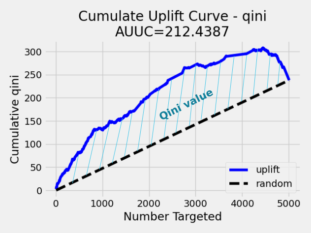
Qini value is calculated as the difference between the Qini AUUC and area under the random uplift curve (random AUUC). The random AUUC is computed as diagonal from zero to overall gain uplift. See the plot below.
Average Excess Cumulative Uplift (AECU)
The Qini value can be generalized for all AUUC metric types. So AECU for Qini metric is the same as Qini value, but the AECU can be also calculated for Gain and Lift metric type. These values are stored in aecu_table.
Partial dependence plot (PDP)
A partial dependence plot gives a graphical depiction of the marginal effect of a variable on the response. The effect of a variable is measured in change in the mean response.
You can plot the partial plot for the whole dataset. However, plotting for treatment and control groups separately could provide better insight into model interpretability. See the Example section below.
Variable Importance
The Variable Importance is calculated based on Uplift Gain improvement. After every split the local split improvement is calculated as difference between Uplift Gain before split and Uplift Gain after split.
The Uplift Gain is calculated based on selected uplift_metric. The higher Uplift Gain the better.
Examples
Below is a simple example showing how to build an Uplift Random Forest model and see its metrics:
library(h2o)
h2o.init()

# Import the uplift dataset into H2O:
data <- h2o.importFile("https://s3.amazonaws.com/h2o-public-test-data/smalldata/uplift/criteo_uplift_13k.csv")

# Set the predictors, response, and treatment column:
# set the predictors
predictors <- c("f1", "f2", "f3", "f4", "f5", "f6","f7", "f8")
# set the response as a factor
data$conversion <- as.factor(data$conversion)
# set the treatment column as a factor
data$treatment <- as.factor(data$treatment)

# Split the dataset into a train and valid set:
data_split <- h2o.splitFrame(data = data, ratios = 0.8, seed = 1234)
train <- data_split[[1]]
valid <- data_split[[2]]

# Build and train the model:
uplift.model <- h2o.upliftRandomForest(training_frame = train,
                                       validation_frame=valid,
                                       x=predictors,
                                       y="conversion",
                                       ntrees=10,
                                       max_depth=5,
                                       treatment_column="treatment",
                                       uplift_metric="KL",
                                       min_rows=10,
                                       seed=1234,
                                       auuc_type="qini")
# Variable importance
varimp <- h2o.varimp(uplift.model)
print(varimp)

# Eval performance:
perf <- h2o.performance(uplift.model)

# Generate predictions on a validation set (if necessary)
predict <- h2o.predict(uplift.model, newdata = valid)

# Plot Uplift Curve
plot(perf, metric="gain")

# Plot Normalized Uplift Curve
plot(perf, metric="gain", normalize=TRUE)

# Get default AUUC value
print(h2o.auuc(perf))

# Get AUUC value by AUUC type (metric)
print(h2o.auuc(perf, metric="lift"))

# Get normalized AUUC value by AUUC type (metric)
print(h2o.auuc_normalized(perf, metric="lift"))

# Get all AUUC types in a table
print(h2o.auuc_table(perf))

# Get threshold and metric scores
print(h2o.thresholds_and_metric_scores(perf))

# Get Qini value
print(h2o.qini(perf))

# Get AECU value
print(h2o.aecu(perf))

# Get all AECU values in a table
print(h2o.aecu_table(perf))

# Plot Partial dependence for valid data
h2o.partialPlot(uplift.model, valid, c("f3"))

mask <- test[, "treatment"] == 1

# Partial dependence plot for treatment group valid data
valid.tr <- valid[mask, ]
h2o.partialPlot(uplift.model, valid.tr, c("f3"))

# Partial dependence plot for control group valid data
valid.ct <- test[!mask, ]
h2o.partialPlot(model, valid.ct, c("f3"))
import h2o
from h2o.estimators import H2OUpliftRandomForestEstimator
h2o.init()

# Import the cars dataset into H2O:
data = h2o.import_file("https://s3.amazonaws.com/h2o-public-test-data/smalldata/uplift/criteo_uplift_13k.csv")

# Set the predictors, response, and treatment column:
predictors = ["f1", "f2", "f3", "f4", "f5", "f6","f7", "f8"]
# set the response as a factor
response = "conversion"
data[response] = data[response].asfactor()
# set the treatment as a factor
treatment_column = "treatment"
data[treatment_column] = data[treatment_column].asfactor()

# Split the dataset into a train and valid set:
train, valid = data.split_frame(ratios=[.8], seed=1234)

# Build and train the model:
uplift_model = H2OUpliftRandomForestEstimator(ntrees=10,
                                              max_depth=5,
                                              treatment_column=treatment_column,
                                              uplift_metric="KL",
                                              min_rows=10,
                                              seed=1234,
                                              auuc_type="qini")
uplift_model.train(x=predictors,
                   y=response,
                   training_frame=train,
                   validation_frame=valid)

# Variable Importance
varimp = uplift_model.varimp()
print(varimp)

# Eval performance:
perf = uplift_model.model_performance()

# Generate predictions on a validation set (if necessary)
pred = uplift_model.predict(valid)

# Plot Uplift curve from performance
perf.plot_uplift(metric="gain", plot=True)

# Plot Normalized Uplift Curve from performance
perf.plot_uplift(metric="gain", plot=True, normalize=True)

# Get default AUUC (in this case Qini AUUC because auuc_type=qini)
print(perf.auuc())

# Get AUUC value by AUUC type (metric)
print(perf.auuc(metric="lift"))

# Get normalized AUUC value by AUUC type (metric)
print(perf.auuc_normalized(metric="lift"))

# Get all AUUC values in a table
print(perf.auuc_table())

# Get thresholds and metric scores
print(perf.thresholds_and_metric_scores())

# Get Qini value
print(perf.qini())

# Get AECU value
print(perf.aecu())

# Get AECU values in a table
print(perf.aecu_table())

# Partial dependence plot for valid data
uplift_model.partial_plot(valid_h2o, cols=["f1"])

mask = valid_h2o[treatment_column] == 1

# Partial dependence plot for treatment group valid data
treatment_valid_h2o = valid[mask, :]
uplift_model.partial_plot(treatment_valid_h2o, cols=["f1"])

# Partial dependence plot for control group valid data
control_valid_h2o = valid[~mask, :]
uplift_model.partial_plot(control_valid_h2o, cols=["f1"])
FAQ
How does the algorithm handle missing values during training?
Missing values are interpreted as containing information (i.e. missing for a reason), rather than missing at random. During tree building, split decisions for every node are found by minimizing the loss function and treating missing values as a separate category that can go either left or right.
Note: Unlike in GLM, in DRF as well as in Uplift DRF numerical values are handled the same way as categorical values. Missing values are not imputed with the mean, as is done by default in GLM.
How does the algorithm handle missing values during testing?
During scoring, missing values follow the optimal path that was determined for them during training (minimized loss function).
What happens if the response has missing values?
No errors will occur, but nothing will be learned from rows containing missing values in the response column.
What happens when you try to predict on a categorical level not seen during training?
Uplift DRF converts a new categorical level to a NA value in the test set, and then splits left on the NA value during scoring. The algorithm splits left on NA values because, during training, NA values are grouped with the outliers in the left-most bin.
Does it matter if the data is sorted?
No.
Should data be shuffled before training?
No.
What if there are a large number of columns?
Uplift DRFs are best for datasets with fewer than a few thousand columns.
What if there are a large number of categorical factor levels?
Large numbers of categoricals are handled very efficiently - there is never any one-hot encoding.
Does the algo stop splitting when all the possible splits lead to worse error measures?
It does if you use
min_split_improvement(which is turned ON by default (0.00001).) When properly tuned, this option can help reduce overfitting.
When does the algo stop splitting on an internal node?
A single tree will stop splitting when there are no more splits that satisfy the minimum rows parameter, if it reaches
max_depth, or if there are no splits that satisfy themin_split_improvementparameter.
How does Uplift DRF decide which feature to split on?
It splits on the column and level that results in the highest uplift gain (based on
uplift_metricparameter type) in the subtree at that point. It considers all fields available from the algorithm. Note that any use of column sampling and row sampling will cause each decision to not consider all data points, and that this is on purpose to generate more robust trees. To find the best level, the histogram binning process is used to quickly compute the potential uplift gain of each possible split. The number of bins is controlled vianbins_catsfor categoricals, the pair ofnbins(the number of bins for the histogram to build, then split at the best point), andnbins_top_level(the minimum number of bins at the root level to use to build the histogram). This number will then be decreased by a factor of two per level.For
nbins_top_level, higher = more precise, but potentially more prone to overfitting. Higher also takes more memory and possibly longer to run.
What is the difference between
nbinsandnbins_top_level?
nbinsandnbins_top_levelare both for numerics (real and integer).nbins_top_levelis the number of bins Uplift DRF uses at the top of each tree. It then divides by 2 at each ensuing level to find a new number.nbinscontrols when Uplift DRF stops dividing by 2.
How is variable importance calculated for Uplift DRF?
Variable importance is not supported for Uplift DRF.
How is column sampling implemented for Uplift DRF?
For an example model using:
100 columns
col_sample_rate_per_treeis 0.602
mtriesis -1 or 7 (refers to the number of active predictor columns for the dataset)For each tree, the floor is used to determine the number of columns that are randomly picked (for this example, (0.602*100)=60 out of the 100 columns).
For classification cases where
mtries=-1, the square root is randomly chosen for each split decision (out of the total 60 - for this example, (\(\sqrt{100}\) = 10 columns).
mtriesis configured independently ofcol_sample_rate_per_tree, but it can be limited by it. For example, ifcol_sample_rate_per_tree=0.01, then there’s only one column left for each split, regardless of how large the value formtriesis.
Why does performance appear slower in Uplift DRF than in GBM?
With DRF as well as Uplift DRF, depth and size of trees can result in speed tradeoffs.
By default, Uplift DRF will go to depth 20, which can lead to up to 1+2+4+8+…+2^19 ~ 1M nodes to be split, and for every one of them, mtries=sqrt(4600)=67 columns need to be considered for splitting. This results in a total work of finding up to 1M*67 ~ 67M split points per tree. Usually, many of the leaves don’t go to depth 20, so the actual number is less. (You can inspect the model to see that value.)
By default, GBM will go to depth 5, so there’s only 1+2+4+8+16 = 31 nodes to be split, and for every one of them, all 4600 columns need to be considered. This results in a total work of finding up to 31*4600 ~ 143k split points (often all are needed) per tree.
This is why the shallow depth of GBM is one of the reasons it’s great for wide (for tree purposes) datasets. To make Uplift DRF faster, consider decreasing
max_depthand/ormtriesand/orntrees.For both algorithms, finding one split requires a pass over one column and all rows. Assume a dataset with 250k rows and 500 columns. GBM can take minutes, while Uplift DRF may take hours. This is because:
Assuming the above, GBM needs to pass over up to 31*500*250k = 4 billion numbers per tree, and assuming 50 trees, that’s up to (typically equal to) 200 billion numbers in 11 minutes, or 300M per second, which is pretty fast;
Uplift DRF needs to pass over up to 1M*22*250k = 5500 billion numbers per tree, and assuming 50 trees, that’s up to 275 trillion numbers, which can take a few hours.
Uplift trees modeling sources:
P. D. Surry, and N. J. Radcliffe, “Quality measures for uplift models”, 2011.