Driverless AI - Training Time Series Model

The purpose of this notebook is to show an example of using Driverless AI to train a time series model. Our goal will be to forecast the Weekly Sales for a particular Store and Department for the next week. The data used in this notebook is from the: Walmart Kaggle Competition where features.csv and train.csv have been joined together.

Here is the Python Client Documentation.

Workflow

1. Import data into Python

2. Format data for Time Series

3. Upload data to Driverless AI

4. Launch Driverless AI Experiment

5. Evaluate model performance

import pandas as pd
import driverlessai

%matplotlib inline
import matplotlib.pyplot as plt
import matplotlib.dates as mdates

Step 1: Import Data

We will begin by importing our data using pandas. We are going to first work with the data in Python to correctly format it for a Driverless AI time series use case.

sales_data = pd.read_csv('./walmart.csv')
sales_data.head()

	Unnamed: 0	Store	Date	IsHoliday	Dept	Weekly_Sales	Temperature	Fuel_Price	MarkDown1	MarkDown2	MarkDown3	MarkDown4	MarkDown5	CPI	Unemployment	Type	Size
0	1	1	2010-02-05	False	1.0	24924.50	42.31	2.572	NaN	NaN	NaN	NaN	NaN	211.096358	8.106	A	151315
1	2	1	2010-02-05	False	26.0	11737.12	42.31	2.572	NaN	NaN	NaN	NaN	NaN	211.096358	8.106	A	151315
2	3	1	2010-02-05	False	17.0	13223.76	42.31	2.572	NaN	NaN	NaN	NaN	NaN	211.096358	8.106	A	151315
3	4	1	2010-02-05	False	45.0	37.44	42.31	2.572	NaN	NaN	NaN	NaN	NaN	211.096358	8.106	A	151315
4	5	1	2010-02-05	False	28.0	1085.29	42.31	2.572	NaN	NaN	NaN	NaN	NaN	211.096358	8.106	A	151315

# Convert Date column to datetime
sales_data["Date"] = pd.to_datetime(sales_data["Date"], format="%Y-%m-%d")
sales_data.head()

	Unnamed: 0	Store	Date	IsHoliday	Dept	Weekly_Sales	Temperature	Fuel_Price	MarkDown1	MarkDown2	MarkDown3	MarkDown4	MarkDown5	CPI	Unemployment	Type	Size
0	1	1	2010-02-05	False	1.0	24924.50	42.31	2.572	NaN	NaN	NaN	NaN	NaN	211.096358	8.106	A	151315
1	2	1	2010-02-05	False	26.0	11737.12	42.31	2.572	NaN	NaN	NaN	NaN	NaN	211.096358	8.106	A	151315
2	3	1	2010-02-05	False	17.0	13223.76	42.31	2.572	NaN	NaN	NaN	NaN	NaN	211.096358	8.106	A	151315
3	4	1	2010-02-05	False	45.0	37.44	42.31	2.572	NaN	NaN	NaN	NaN	NaN	211.096358	8.106	A	151315
4	5	1	2010-02-05	False	28.0	1085.29	42.31	2.572	NaN	NaN	NaN	NaN	NaN	211.096358	8.106	A	151315

Step 2: Format Data for Time Series

The data has one record per Store, Department, and Week. Our goal for this use case will be to forecast the total sales for the next week.

The only features we should use as predictors are ones that we will have available at the time of scoring. Features like the Temperature, Fuel Price, and Unemployment will not be known in advance. Therefore, before we start our Driverless AI experiments, we will choose to use the previous week’s Temperature, Fuel Price, Unemployment, and CPI attributes. This information we will know at time of scoring.

lag_variables = ["Temperature", "Fuel_Price", "CPI", "Unemployment"]
dai_data = sales_data.set_index(["Date", "Store", "Dept"])
lagged_data = dai_data.loc[:, lag_variables].groupby(level=["Store", "Dept"]).shift(1)

# Join lagged predictor variables to training data
dai_data = dai_data.join(lagged_data.rename(columns=lambda x: x +"_lag"))

# Drop original predictor variables - we do not want to use these in the model
dai_data = dai_data.drop(lagged_data, axis=1)
dai_data = dai_data.reset_index()

dai_data.head()

	Date	Store	Dept	Unnamed: 0	IsHoliday	Weekly_Sales	MarkDown1	MarkDown2	MarkDown3	MarkDown4	MarkDown5	Type	Size	Temperature_lag	Fuel_Price_lag	CPI_lag	Unemployment_lag
0	2010-02-05	1	1.0	1	False	24924.50	NaN	NaN	NaN	NaN	NaN	A	151315	NaN	NaN	NaN	NaN
1	2010-02-05	1	26.0	2	False	11737.12	NaN	NaN	NaN	NaN	NaN	A	151315	NaN	NaN	NaN	NaN
2	2010-02-05	1	17.0	3	False	13223.76	NaN	NaN	NaN	NaN	NaN	A	151315	NaN	NaN	NaN	NaN
3	2010-02-05	1	45.0	4	False	37.44	NaN	NaN	NaN	NaN	NaN	A	151315	NaN	NaN	NaN	NaN
4	2010-02-05	1	28.0	5	False	1085.29	NaN	NaN	NaN	NaN	NaN	A	151315	NaN	NaN	NaN	NaN

Now that our training data is correctly formatted, we can run a Driverless AI experiment to forecast the next week’s sales.

Step 3: Upload Data to Driverless AI

We will split out data into two pieces: training and test (which consists of the last week of data).

train_data = dai_data.loc[dai_data["Date"] < "2012-09-28"]
test_data = dai_data.loc[dai_data["Date"] == "2012-09-28"]

To upload the datasets, we will sign into Driverless AI.

address = 'http://ip_where_driverless_is_running:12345'
username = 'username'
password = 'password'
dai = driverlessai.Client(address = address, username = username, password = password)
# make sure to use the same user name and password when signing in through the GUI

train_path = "./train_data.csv"
test_path = "./test_data.csv"

train_data.to_csv(train_path, index = False)
test_data.to_csv(test_path, index = False)

# Add datasets to Driverless AI
train_data = dai.datasets.create(
    data=train_path,
    data_source='upload',
    name='walmart-example-train'
)
test_data = dai.datasets.create(
    data=test_path,
    data_source='upload',
    name='walmart-example-test'
)

Complete 100.00% - [4/4] Computing column statistics
Complete 100.00% - [4/4] Computing column statistics

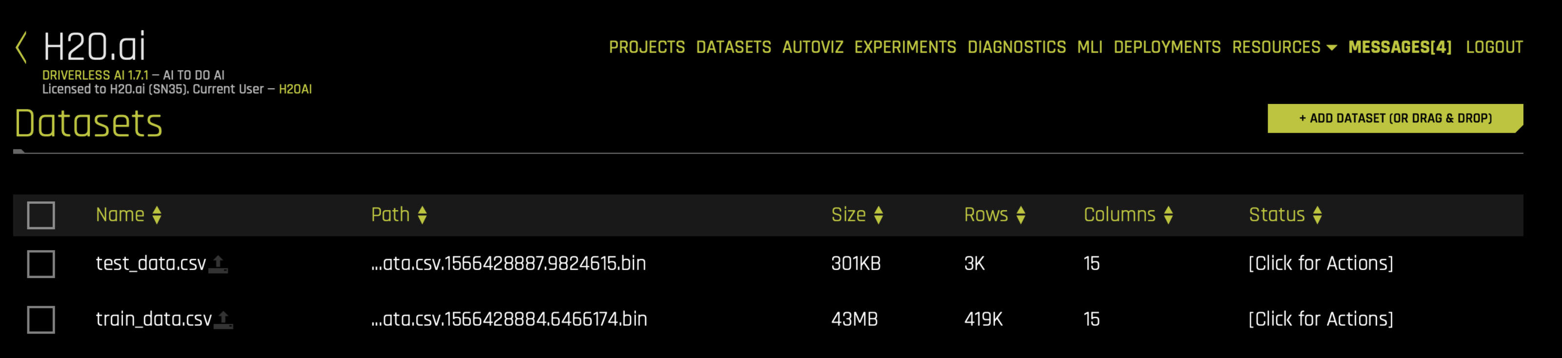
Equivalent Steps in Driverless: Uploading Train & Test CSV Files

Step 4: Launch Driverless AI Experiment

We will now launch the Driverless AI experiment. To do that we will need to specify the parameters for our experiment. Some of the parameters include:

• Target Column: The column we are trying to predict.

• Dropped Columns: The columns we do not want to use as predictors such as ID columns, columns with data leakage, etc.

• Is Time Series: Whether or not the experiment is a time-series use case.

• Time Column: The column that contains the date/date-time information.

• Time Group Columns: The categorical columns that indicate how to group the data so that there is one time series per group. In our example, our Time Groups Columns are Store and Dept. Each Store and Dept, corresponds to a single time series.

• Number of Prediction Periods: How far in the future do we want to predict?

• Number of Gap Periods: After how many periods can we start predicting? If we assume that we can start forecasting right after the training data ends, then the Number of Gap Periods will be 0.

For this experiment, we want to forecast next week’s sales for each Store and Dept. Therefore, we will use the following time series parameters:

• Time Group Columns: [Store, Dept]

• Number of Prediction Periods: 1 (a.k.a., horizon)

• Number of Gap Periods: 0

Note that the period size is unknown to the Python client. To overcome this, you can also specify the optional time_period_in_seconds parameter, which can help specify the horizon in real time units. If this parameter is omitted, Driverless AI will automatically detect the period size in the experiment, and the horizon value will respect this period. I.e., if you are sure your data has 1 week period, you can say num_prediction_periods=14, otherwise it is possible that the model may not work out correctly.

experiment = dai.experiments.create(name='walmart_time_series',
                                    test_dataset=test_data,
                                    train_dataset=train_data,
                                    task='regression',
                                    target_column='Weekly_Sales',
                                    drop_columns=['sample_weight'],
                                    time_column= 'Date',
                                    scorer='RMSE',
                                    accuracy=5,
                                    time=3,
                                    interpretability=5,
                                    num_prediction_periods=1,
                                    num_gap_periods=0,
                                    time_groups_columns = ['Store', 'Dept'],
                                    seed=1234)

Experiment launched at: http://localhost:12345/#experiment?key=9f376088-408b-11eb-b9de-0242ac110002
Complete 100.00% - Status: Complete

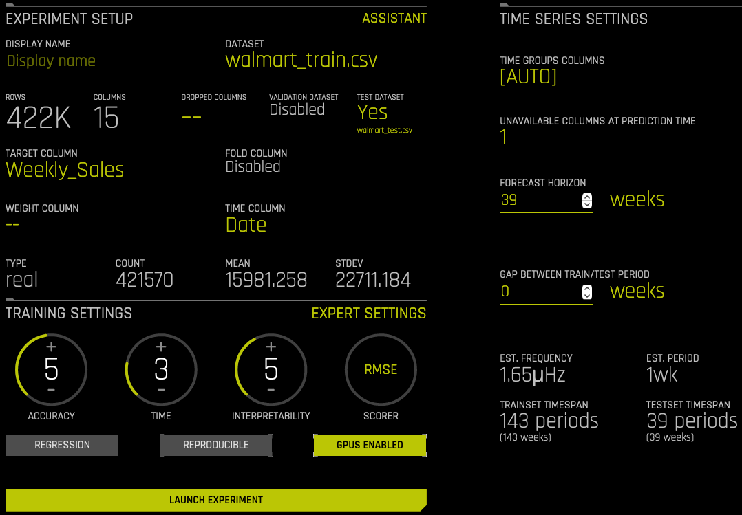
Equivalent Steps in Driverless: Launching Driverless AI Experiment

Step 5. Evaluate Model Performance

Now that our experiment is complete, we can view the model performance metrics within the experiment object.

metrics = experiment.metrics()
print("Validation RMSE: ${:,.0f}".format(metrics['val_score']))
print("Test RMSE: ${:,.0f}".format(metrics['test_score']))

Validation RMSE: $2,425
Test RMSE: $2,084

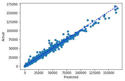
We can also plot the actual versus predicted values from the test data.

target="Weekly_Sales"
prediction = experiment.predict(test_data, [target])
path = prediction.download('')

forecast_predictions = pd.read_csv(path)
forecast_predictions.head()

Complete
Downloaded '9f376088-408b-11eb-b9de-0242ac110002_preds_f6e2264e.csv'

	Weekly_Sales	Weekly_Sales.predicted
0	14734.64	12660.375000
1	1163.75	1384.219238
2	1773.32	1579.065430
3	27205.40	29764.876953
4	4390.19	4197.859863

plt.scatter(forecast_predictions['Weekly_Sales.predicted'], forecast_predictions['Weekly_Sales'])
plt.plot([0, max(forecast_predictions['Weekly_Sales.predicted'])],[0, max(forecast_predictions['Weekly_Sales'])], 'b--',)
plt.xlabel("Predicted")
plt.ylabel("Actual")
plt.show()

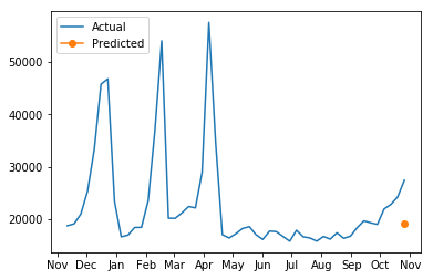
Lastly, we can download the test predictions from Driverless AI and examine the forecasted sales vs actual for a selected store and department.

test_data = pd.read_csv('./test_data.csv')
selected_ts = sales_data.loc[(sales_data["Store"] == 1) & (sales_data["Dept"] == 1)].tail(n = 51)

selected_ts_forecast = forecast_predictions.loc[(test_data["Store"] == 1) &
                                                (test_data["Dept"] == 1)]

# Plot the forecast of a select store and department
years = mdates.MonthLocator()
yearsFmt = mdates.DateFormatter('%b')

fig, ax = plt.subplots()

ax.plot(selected_ts["Date"], selected_ts["Weekly_Sales"], label = "Actual")
ax.plot(selected_ts["Date"].iloc[-1], selected_ts_forecast["Weekly_Sales.predicted"], marker='o', label = "Predicted")

ax.xaxis.set_major_locator(years)
ax.xaxis.set_major_formatter(yearsFmt)
plt.legend(loc='upper left')
plt.show()