Concepts
Custom Recipe to Improve Predictions
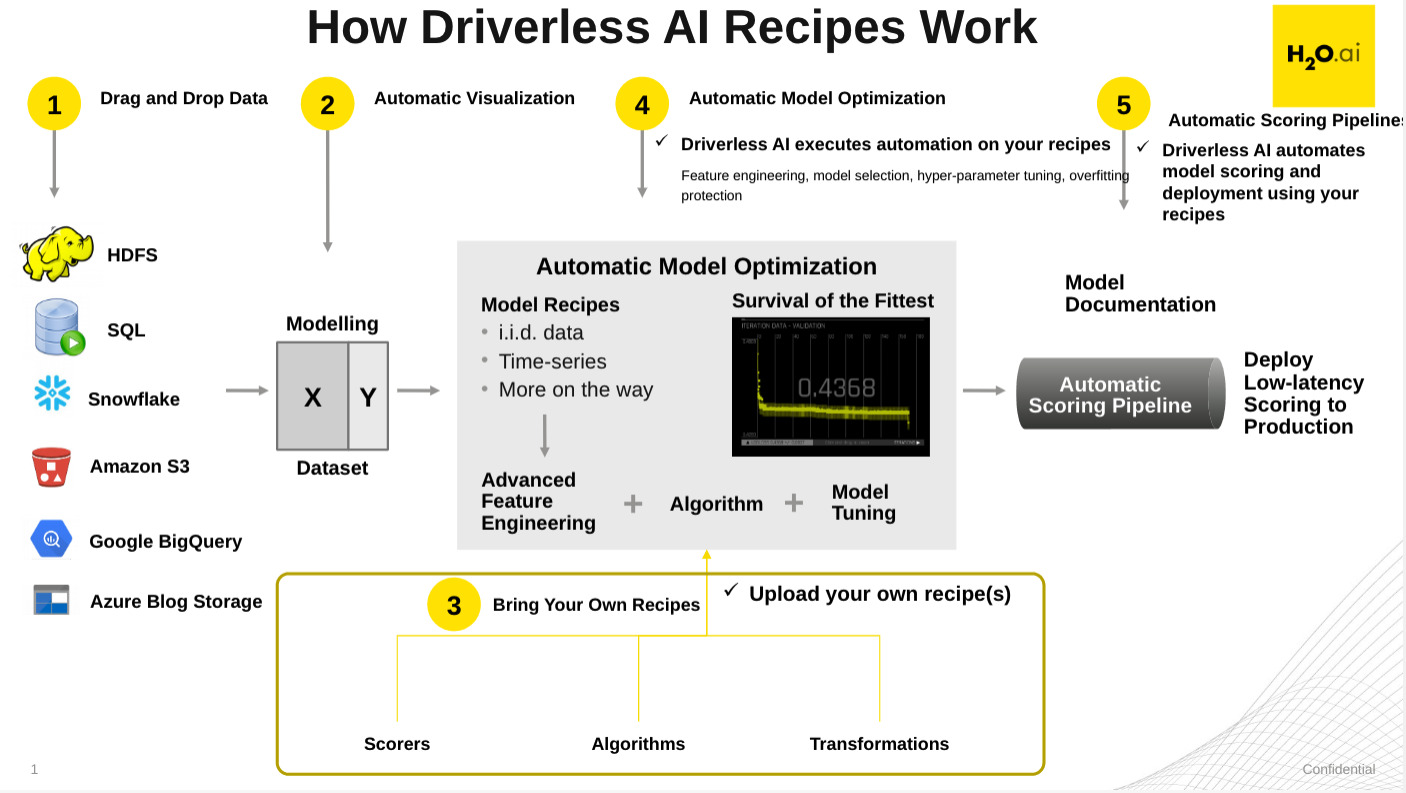
The latest versions of Driverless AI implement a key feature called BYOR[1], which stands for Bring Your Own Recipes, and was introduced with Driverless AI (1.7.0). This feature has been designed to enable Data Scientists or domain experts to influence and customize the machine learning optimization used by Driverless AI as per their business needs. This additional feature engineering technique is aimed at improving the accuracy of the model.
Recipes are customizations and extensions to the Driverless AI platform. They are nothing but Python code snippets uploaded into Driverless AI at runtime, like plugins. Recipes can be either one or a combination of the following:
- Custom machine learning models
- Custom scorers (classification or regression)
- Custom transformers
Machine learning
Machine learning is a subset of Artificial Intelligence (AI) where the focus is to create machines that can simulate human intelligence. One critical distinction between artificial intelligence and machine learning is that machine learning models "learn" from the data the models get exposed to. A machine learning algorithm trains on a dataset to make predictions. These predictions are, at times, used to optimize a system or assist with decision-making.
Machine learning training
Advances in technology have made it easier for data to be collected and made available. The available type of data will determine the kind of training that the machine learning model can undergo. There are two types of machine learning training, supervised and unsupervised learning. Supervised learning is when the dataset contains the output that you are trying to predict. For cases where the predicting variable is not present, unsupervised learning can be used. Both types of training define the relationship between input and output variables.
In machine learning, the input variables are called features and the output variables are called labels. The labels, in this case, are what we are trying to predict. The goal is to take the inputs/variables/features and use them to come up with predictions on never-before-seen data. In linear regression, the features are the x-variables, and the labels are the y-variables. An example of a label could be the future price of avocados.
A machine learning model defines the relationship between features and labels. Anyone can train a model by feeding it examples of particular instances of data. You can have two types of examples: labeled and unlabeled. Labeled examples are those where the X and Y values (features, labels) are known. Unlabeled examples are those where we know the X value, but we don't know the Y value. Your dataset is similar to an example; the columns that will be used for training are the features; the rows are the instances of those features. The column that you want to predict is the label.
Supervised learning takes labeled examples and allows a model that is being trained to learn the relationship between features and labels. The trained model can then be used on unlabelled data to predict the missing Y value. The model can be tested with either labeled or unlabeled data. Note that H2O Driverless AI creates models with labeled examples.
Data preparation
A machine learning model is as good as the data that is used to train it. If you use garbage data to train your model, you will get a garbage model. With that said, before uploading a dataset into tools that will assist you with building your machine learning model (such as Driverless AI), ensure that the dataset has been cleaned and prepared for training. Transforming raw data into another format, which is more appropriate and valuable for analytics, is called data wrangling.
Data wrangling can include extractions, parsing, joining, standardizing, augmenting, cleansing, and consolidating until the missing data is fixed or removed. Data preparation includes the dataset being in the correct format for what you are trying to do; accordingly, duplicates are removed, missing data is fixed or removed, and finally, categorical values are transformed or encoded to a numerical type.
Data wrangling can be done in H2O Driverless AI via a data recipe, the JDBC connector or through live code which will create a new dataset by modifying the existing one.
Data transformation / feature engineering
Data transformation or feature engineering is the process of creating new features (input variables) from the existing ones. Proper data transformations on a dataset can include scaling, decomposition, and aggregation. Some data transformations include looking at all the features and identifying which features can be combined to make new ones that will be more useful to the model's performance. For categorical features, the recommendation is for classes that have few observations to be grouped to reduce the likelihood of the model overfitting. Categorical features may be converted to numerical representations since many algorithms cannot handle categorical features directly. Besides, data transformation removes features that are not used or are redundant. These are only a few suggestions when approaching feature engineering. Feature engineering is very time-consuming due to its repetitive nature; it can also be costly. After successfully having a notion of well-done data transformation, the next step in creating a model is selecting an algorithm.
Algorithm selection
Machine learning algorithms are computational functions that enable computers to automatically learn patterns and relationships from the data and the given input variables, and then make predictions or decisions based on that learning. In supervised learning, there are many algorithms to select from for training. The type of algorithm(s) will depend on the size of your dataset, structure, and the type of problem you are trying to solve. Through trial and error, the best performing algorithms can be found for your dataset.
Model training
Datasets
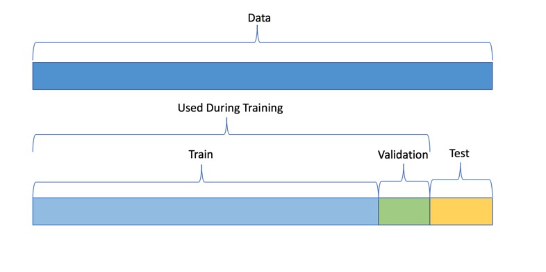
When training a machine learning model, one good practice is to split up your dataset into subsets: training, validation, and testing sets. A good ratio for the entire dataset is 70-15-15, 70% of the whole dataset for training, 15% for validation, and the remaining 15% for testing. The training set is the data used to train the model, and it needs to be big enough to get significant results from it. The validation set is the data held back from the training and will be used to evaluate and adjust the trained model's hyperparameters and, hence, adjust the performance. Finally, the test set is data that has also been held back and will be used to confirm the final model's results.
The validation dataset is used for tuning the modeling pipeline. If provided, the entire training data will be used for training, and validation of the modeling pipeline is performed with only this validation dataset. When you do not include a validation dataset, Driverless AI will do K-fold cross-validation for I.I.D. (identically and independently distributed) experiments and multiple rolling window validation splits for time series experiments. For this reason, it is not generally recommended to include a validation dataset as you are then validating on only a single dataset. Note that time series experiments cannot be used with a validation dataset: including a validation dataset will disable the ability to select a time column and vice versa.
This dataset must have the same number of columns (and column types) as the training dataset. Also, note that if provided, the validation set is not sampled down, so it can lead to large memory usage, even if accuracy=1 (which reduces the train size). In a moment, we will learn more about accuracy when preparing an experiment.
Another part of model training is fitting and tuning the models. For fitting and tuning, hyperparameters need to be tuned, and cross-validation needs to take place using only the training data. Various hyperparameter values will need to be tested. "A hyperparameter is a parameter that is set before the learning process begins. These parameters are tunable and can directly affect how well a model trains. The hyperparameter value is used to determine the rate at which the model learns.
With cross-validation, the whole dataset is utilized, and each model is trained on a different subset of the training data. Additionally, a cross-validation loop will be set to calculate the cross-validation score for each set of hyperparameters for each algorithm. Based on the cross-validation score and hyperparameter values, you can select the model for each algorithm that has been tuned with training data and tested with your test set.
Automated Machine Learning
AutoML or Automated Machine Learning is the process of automating algorithm selection, feature generation, hyperparameter tuning, iterative modeling, and model assessment. AutoML tools such as H2O Driverless AI make it easy to train and evaluate machine learning models. Automating the repetitive tasks around Machine Learning development allows individuals to focus on the data and the business problems they are trying to solve.
ROC - Receiver Operating Characteristics
This type of graph is called a Receiver Operating Characteristic curve (or ROC curve). You will most likely see this graph in H2O Driverless AI, when exploring your experiment results and viewing the experiment summary. It is a plot of the true positive rate against the false-positive rate for the different possible cut points of a diagnostic test.
A ROC curve is a useful tool because it only focuses on how well the model was able to distinguish between classes with the help of the Area Under the Curve (AUC). However, for models where one of the classes occurs rarely, a high AUC could provide a false sense that the model is correctly predicting the results. This is where the notion of precision and recall become essential.
Prec-Recall: Precision-Recall Graph
Prec-Recall is a complementary tool to ROC curves, especially when the dataset has a significant skew. You will most likely see this plot in H2O Driverless AI, when exploring your experiment results and viewing the experiment summary. The Prec-Recall curve plots the precision or positive predictive value (y-axis) versus sensitivity or true positive rate (x-axis) for every possible classification threshold. At a high level, we can think of precision as a measure of exactness or quality of the results while recall as a measure of completeness or quantity of the results obtained by the model. Prec-Recall measures the relevance of the results obtained by the model.
Cumulative Lift Chart
This chart shows lift stats on validation data. For example, “How many times more observations of the positive target class are in the top predicted 1%, 2%, 10%, etc., (cumulative) compared to selecting observations randomly?” By definition, the Lift at 100% is 1.0. Lift can help answer the question of how much better you can expect to do with the predictive model compared to a random model (or no model). Lift is a measure of the effectiveness of a predictive model calculated as the ratio between the results obtained with a model and with a random model(or no model). In other words, the ratio of gain % to the random expectation % at a given quantile. The random expectation of the xth quantile is x%.
Cumulative Gains Chart
Gain and Lift charts measure a classification model's effectiveness by looking at the ratio between the results obtained with a trained model versus a random model(or no model). The Gain and Lift charts help us evaluate the performance of the classifier as well as answer questions such as what percentage of the dataset captured has a positive response as a function of the selected percentage of a sample. Additionally, we can explore how much better we can expect to do with a built model than a random model(or no model).
For better visualization, the percentage of positive responses compared to a selected percentage sample uses Cumulative Gains and Quantile.
Kolmogorov-Smirnov chart
Kolmogorov-Smirnov or K-S measures classification models' performance by measuring the degree of separation between positives and negatives for validation or test data. The K-S is 100 if the scores partition the population into two separate groups in which one group contains all the positives and the other all the negatives. On the other hand, if the model cannot differentiate between positives and negatives, then it is as if the model selects cases randomly from the population. The K-S would be 0. In most classification models, the K-S will fall between 0 and 100, and the higher the value, the better the model is at separating the positive from negative cases.
K-S or the Kolmogorov-Smirnov chart measures the degree of separation between positives and negatives for validation or test data.
Natural Language Processing Concepts
Natural Language Processing (NLP)
NLP is the field of study that focuses on the interactions between human language and computers. NLP sits at the intersection of computer science, artificial intelligence, and computational linguistics[1]. NLP is a way for computers to analyze, understand, and derive meaning from human language in a smart and useful way. By utilizing NLP, developers can organize and structure knowledge to perform tasks such as:
- Automatic tagging of incoming customer queries related to credit card, loans, etc
- Sentiment analysis of social media reviews
- Using free text variables along with numeric variables for credit risk and fraud models
- Emotion detection
- Profanity detection
The text data is highly unstructured, but the Machine learning algorithms usually work with numeric input features. So before we start with any NLP project, we need to pre-process and normalize the text to make it ideal for feeding into the commonly available Machine learning algorithms. This essentially means we need to build a pipeline of some sort that breaks down the problem into several pieces. We can then apply various methodologies to these pieces and plug the solution together in a pipeline.
Building a Typical NLP Pipeline
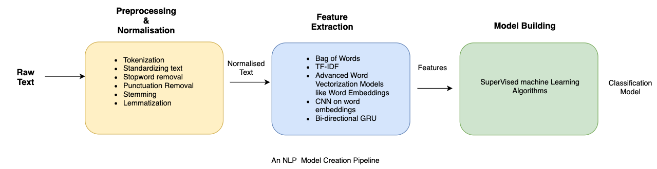
The figure above shows how a typical pipeline looks. It is also important to note that there may be variations depending upon the problem at hand. Hence the pipeline will have to be adjusted to suit our needs. Driverless AI automates the above process. Let's try and understand some of the components of the pipeline in brief:
Text preprocessing
Text pre-processing involves using various techniques to convert raw text into well-defined sequences of linguistic components with standard structure and notation. Some of those techniques are:
Sentence Segmentation: involves identifying sentence boundaries between words in different sentences. Since most written languages have punctuation marks that occur at sentence boundaries, sentence segmentation is frequently referred to as sentence boundary detection, sentence boundary disambiguation, or sentence boundary recognition. All these terms refer to the same task: determining how a text should be divided into sentences for further processing.
Text Tokenization: Tokenization involves splitting raw text corpus into sentences and then further splitting each sentence into words.
Text Standardisation: Once the text has been tokenized, it is normalized by getting rid of the noise. Noise relates to anything that isn't in a standard format like punctuation marks, special characters, or unwanted tokens. If required, case conversions can also be done, i.e., converting all tokens into either lowercase or uppercase.
Removing Stopwords: Stop words are words that appear very frequently in a text like "and", "the", and "a", but appear to be of little value in helping select documents. Therefore, such words are excluded from the vocabulary entirely.
Stemming: Stemming is the process of reducing inflected (or sometimes derived) words to their stem, base, or root form — generally a written word form. For example: if we were to stem the following words: "Stems," "Stemming," "Stemmed," "and "Stemtization," the result would be a single token "stem."
Lemmatization: a similar operation to Stemming is Lemmatization. However, the major difference between the two is that Stemming can often create non-existent words, whereas Lemmatization creates actual words. An example of Lemmatization: "run" is a base form for words like "running" or "ran," and the word "better" and "good" are in the same lemma, so they are considered the same.
It is important to note here that the above steps are not mandatory, and their usage depends upon the use case. For instance, in sentiment analysis, emoticons signify polarity, and stripping them off from the text may not be a good idea. The general goal of Normalization, Stemming, and Lemmatization techniques is to improve the model's generalization. Essentially we are mapping different variants of what we consider to be the same or very similar "word" to one token in our data.
Feature Extraction
The Machine Learning Algorithms usually expect features in the form of numeric vectors. Hence, after the initial preprocessing phase, we need to transform the text into a meaningful vector (or array) of numbers. This process is called feature extraction. Let's see how some of the feature-extracting techniques work.
Bag of Words (BoW): The bag-of-words represents text that describes the occurrence of words within a document. It involves two things:
- A vocabulary of known words
- A measure of the presence of known words
The intuition behind the Bag of Words is that documents are similar if they have identical content, and we can get an idea about the meaning of the document from its content alone.
Example implementation
The following models a text document using bag-of-words here are two simple text documents:
- John likes to watch movies. Mary likes movies too.
- John also likes to watch football games.
Based on these two text documents, a list is constructed as follows for each document:
- "John", "likes" ,"to" ,"watch" ,"movies" ,"Mary" ,"likes","movies" ,"too"
- "John" ,"also" ,"likes" ,"to" ,"watch" ,"football" ,"games"
Representing each bag-of-words as a JSON object and attributing to the respective JavaScript variable:
- BoW1 = {"John":1, "likes":2, "to":1, "watch":1 ,"movies":2 ,"Mary":1 ,"too":1};
- BoW2 = {"John":1, "also":1, "likes":1, "to":1, "watch":1, "football":1, "games":1};
It is important to note that BoW does not retain word order and is sensitive towards document length, i.e., token frequency counts could be higher for longer documents.
It is also possible to create BoW models with consecutive words, also known as n-grams:
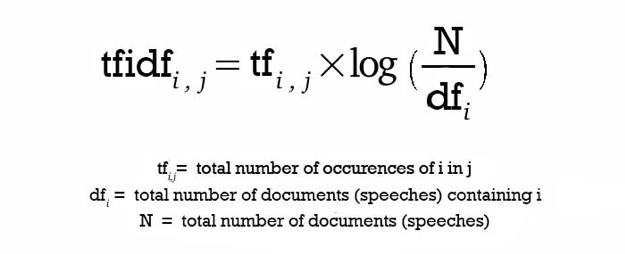
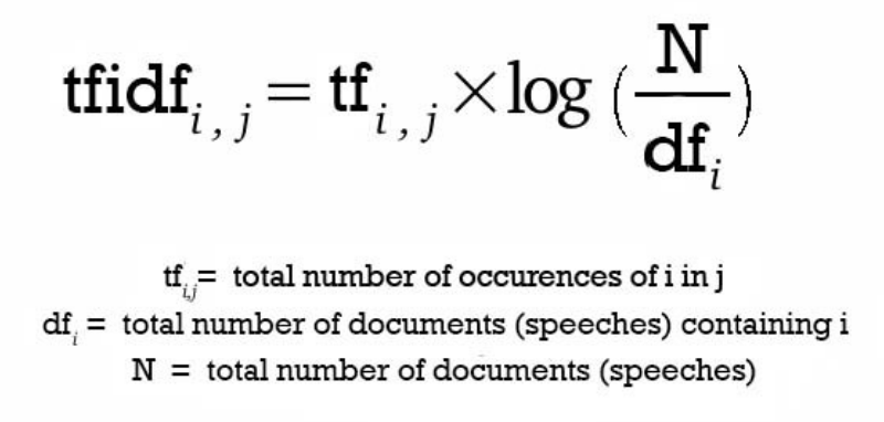
TF-IDF Model: A problem with the Bag of Words approach is that highly frequent words start to dominate in the document (e.g., larger score) but may not contain as much "informational content." Also, it will give more weight to longer documents than shorter ones. One approach is to rescale the frequency of words by how often they appear in all documents so that the scores for frequent words across all documents are penalized. This approach of scoring is called Term Frequency-Inverse Document Frequency, or TF-IDF [2] for short, where:
Term Frequency is a scoring of the frequency of the word in the current document. TF = (Number of times term t appears in a document)/(Number of terms in the document)
Inverse Document Frequency: is a scoring of how rare the word is across documents. IDF = 1+log(N/n), where N is the number of documents, and n is the number of documents a term t has appeared. TF-IDF weight is often used in information retrieval and text mining. This weight is a statistical measure used to evaluate how important a word is to a document in a collection or corpus:
The dimensions of the output vectors are high. This also gives importance to the rare terms that occur in the corpus, which might help our classification tasks:
Principal Component Analysis (PCA):
Principal Component Analysis is a dimension reduction tool that can be used to reduce a large set of variables to a small set that still contains most of the information in the original set.
Truncated SVD:
SVD stands for Singular Value Decomposition[3], which is a way to decompose matrices. Truncated SVD is a common method to reduce the dimension for text-based frequency/vectors.
Advanced Word Vectorization Models:
TFIDF and frequency-based models represent counts and significant word information, but they lack semantics of the words in general. One of the popular representations of text to overcome this is Word Embeddings.
Word embeddings is a feature engineering technique for text where words or phrases from the vocabulary are mapped to vectors of real numbers. There are ways to create more advanced word vectorization models for extracting features from text data like word2vec[2] model. The word2vec model was released in 2013 by Google; word2vec is a neural network-based implementation that learns distributed vector representations of words based on continuous Bag of Words and skip-gram–based architectures.
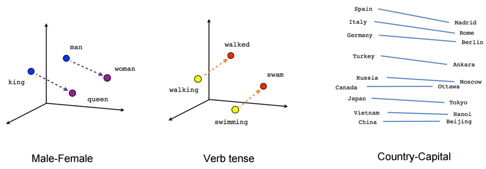
Representations are made so that words that have similar meanings are placed close or equidistant to each other. For example, a word like king is closely associated with queen in this vector representation.
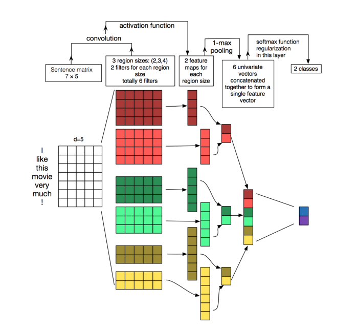
Convolution Neural Network (CNN) Models on Word Embeddings:
CNN's are generally used in computer vision; however, they've recently been applied on top of pre-trained word vectors for sentence-level classification tasks, and the results were promising[5].
Word embeddings can be passed as inputs to CNN models, and cross-validated predictions are obtained from them. These predictions can then be used as a new set of features.
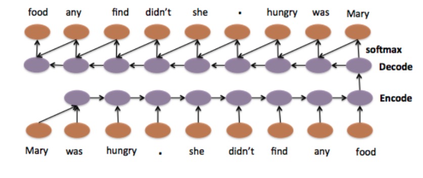
Recurrent neural networks
RNNs like LSTM and GRU are state-of-the-art algorithms for NLP problems. A Bi-directional GRU model is putting two independent RNN models in one.
For example, in the sentence "John is walking on the golf court," a unidirectional model would represent states representing "golf" based on "John is walking" but not the "court." In a bi-directional model, the representation would also account for the later representations giving the model more predictive power. This makes it a more natural approach when dealing with textual data since the text is naturally sequential[6].
Transformer-based language models
Transformer-based language models like BERT are state-of-the-art NLP models that can be used for a wide variety of NLP tasks. These models capture the contextual relation between words by using an attention mechanism. Unlike directional models that read text sequentially, a Transformer-based model reads the entire sequence of text at once, allowing it to learn the word's context based on all of its surrounding words. The embeddings obtained by these models show improved results in comparison to earlier embedding approaches.
Building Text Classification Models
Once the features have been extracted, they can then be used for training a classifier.
With this task in mind, let's learn about Driverless AI NLP Recipes.
Driverless AI NLP Recipe
This section will discuss all current NLP model capabilities of Driverless AI. Keep in mind that not all settings discussed below have been enabled in the current sentiment analysis experiment.
Text data can contain critical information to inform better predictions. Driverless AI automatically converts text strings into features using powerful techniques like TFIDF, CNN, and GRU. Driverless AI now also includes state-of-the-art PyTorch BERT transformers. With advanced NLP techniques, Driverless AI can also process larger text blocks, build models using all available data, and solve business problems like sentiment analysis, document classification, and content tagging.
The Driverless AI platform can support both standalone text and text with other columns as predictive features. In particular, the following NLP recipes are available for a given text column:
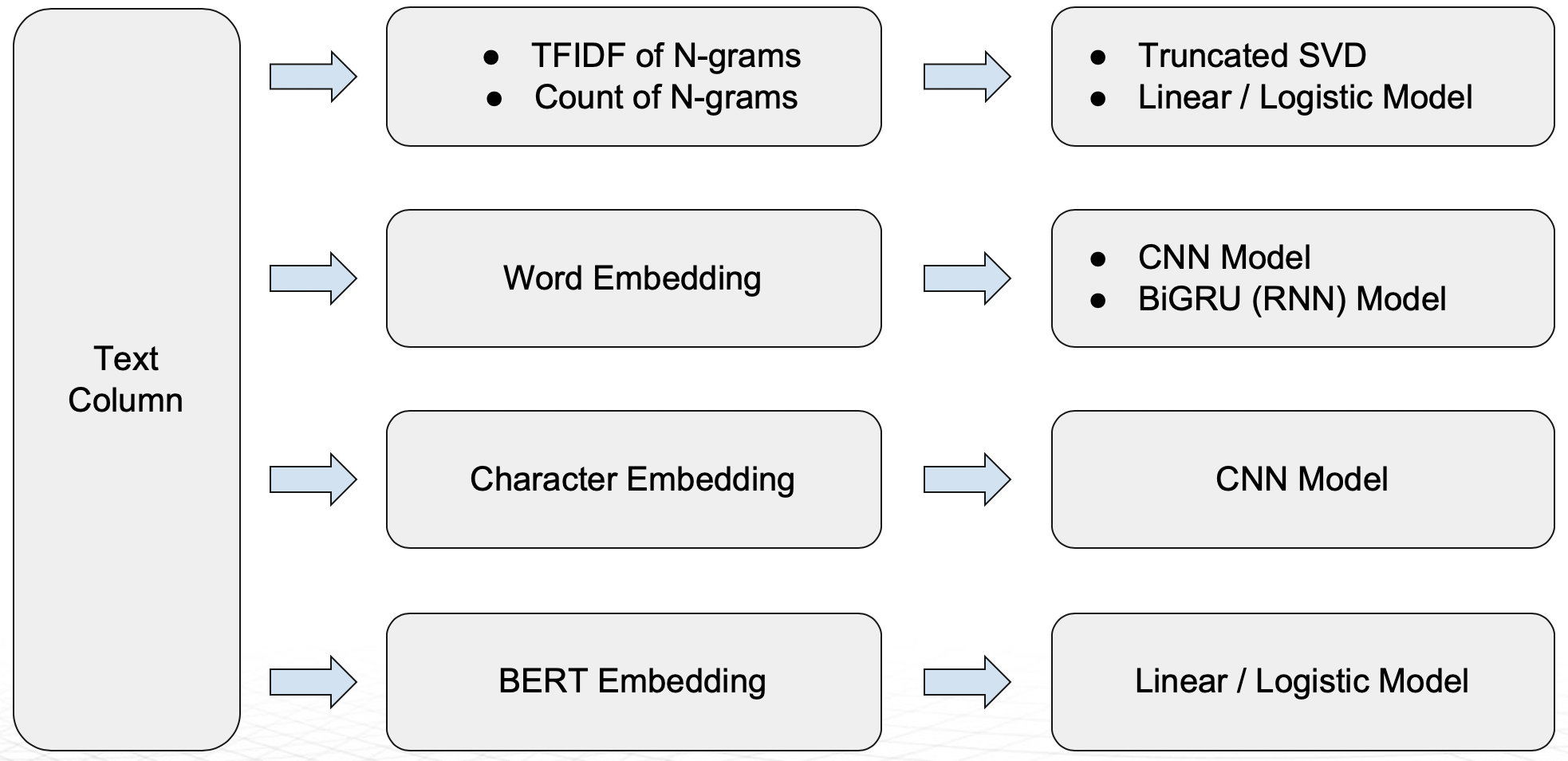
Key Capabilities of Driverless AI NLP Recipes
- N-grams:
- An n-gram is a contiguous sequence of n items from a given text or speech sample.
- TFIDF of n-grams:
- Frequency-based features can be multiplied with the inverse document frequency to get term frequency-inverse document frequency (TF-IDF) vectors. Doing so also gives importance to the rare terms in the corpus, which can help in specific classification tasks.
- Frequency-based features can be multiplied with the inverse document frequency to get term frequency-inverse document frequency (TF-IDF) vectors. Doing so also gives importance to the rare terms in the corpus, which can help in specific classification tasks.
- Frequency of n-grams:
- Frequency-based features represent the count of each word in the given text in the form of vectors. Frequency-based features are created for different n-gram values[2]. The dimensions of the output vectors are quite high. Words and n-grams that occur more times will get higher weightage than the ones that occur less frequently.
- Truncated SVD Features:
- Both TFIDF and Frequency of n-grams result in a higher dimension. To tackle this, we use Truncated SVD to decompose the vector arrays in lower dimensions.
- Linear models on TF/IDF vectors:
- Our NLP recipe also has linear models on top of n-gram TFIDF/ frequency vectors. This captures linear dependencies that are simple yet significant in achieving the best accuracies.
- Word Embeddings:
- Driverless AI NLP recipe uses the power of word embeddings where words or phrases from the vocabulary are mapped to vectors of real numbers.
- Bi-direction GRU models on Word Embeddings (TensorFlow):
- A BI-directional GRU model is like putting independent RNN models in one. GRU gives higher speed and almost similar accuracy when compared to its counterpart LSTM.
- Convolution neural network models on:
- Word embeddings followed by CNN model (TensorFlow):
- In Driverless AI, we pass word embeddings as input to CNN models; we get cross-validated predictions from it and use them as a new set of features.
- Character embeddings followed by CNN model (TensorFlow):
- Natural language processing is complex as the language is hard to understand given small data and different languages. Targeting languages like Japanese, Chinese where characters play a major role, we have character level embeddings in our recipe as well.
- In character embeddings, each character gets represented in the form of vectors rather than words. Driverless AI uses character level embeddings as input to CNN models and later extracts class probabilities to feed as features for downstream models: this gives the ability to work in languages other than English. In languages like Japanese and Chinese, where there is no concept of words, character embeddings will be useful.
- Word embeddings followed by CNN model (TensorFlow):
- BERT/DistilBERT based embeddings for Feature Engineering (PyTorch):
- BERT and DistilBERT models can be used to generate embeddings for any text columns. These pre-trained models are used to get embeddings for the text, followed by Linear/Logistic Regression to generate features that Driverless AI can then use for any downstream models in Driverless AI.
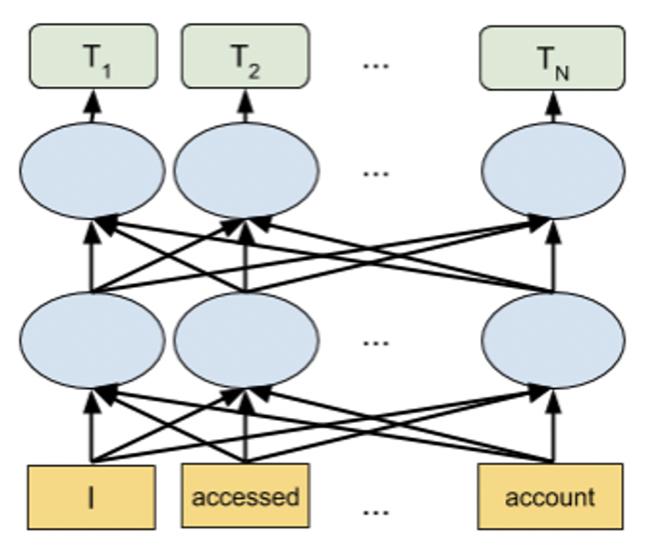
- PyTorch Transformer Architecture Models (e.g., BERT) as Modeling Algorithms:
- With versions of Driverless AI 1.9 and higher, the Transformer-based architectures shown in the diagram below are supported as models in Driverless AI:
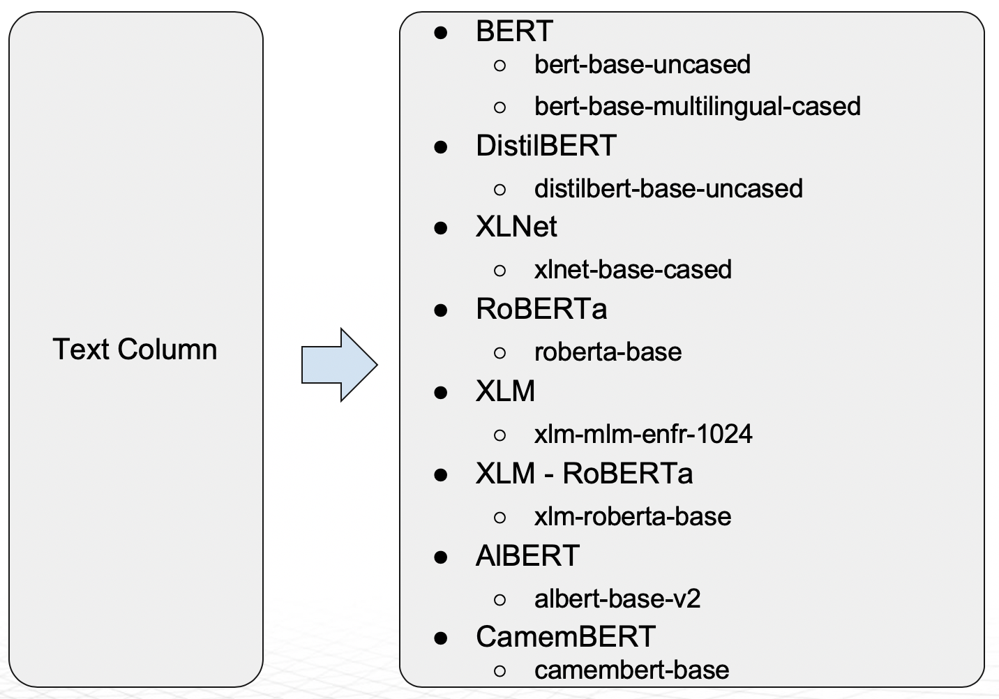
- The BERT model supports multiple languages. DistilBERT is a distilled version of BERT that has fewer parameters compared to BERT (40% less), and it is faster (60% speedup) while retaining 95% of BERT level performance. The DistilBERT model can be helpful when training time and model size is important.
- With versions of Driverless AI 1.9 and higher, the Transformer-based architectures shown in the diagram below are supported as models in Driverless AI:
- Domain Specific BERT Recipes Driverless AI can also extend the DAI Base BERT model for domain-specific problems:
Experiment scoring and analysis concepts
Binary Classifier
A binary classification model is a type of machine learning model that predicts the category (class) to which an element belongs, given a set of options. In our example, the model predicts whether a customer will default on their home loan (positive class) or not default (negative class). The generated model can then be used to classify new customers based on their characteristics.
Understanding Model Errors: False Negatives and False Positives
It's important to consider potential errors made by the model. These errors fall into two categories:
- False Negative: The model predicts a customer will not default on their loan, but they actually do.
- False Positive: The model predicts a customer will default on their loan, but they actually don't.
Confusion Matrix
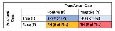
The confusion matrix, also known as the error matrix, is a valuable tool for visualizing a model's classification performance, including its error rate. This table allows you to calculate various metrics, such as error rate, accuracy, specificity, sensitivity, and precision. These metrics provide insights into how well your model performs at classifying or predicting data points.
GINI, ACC, F1 F0.5, F2, MCC and Log Loss
ROC and Prec-Recall curves are extremely useful to test a binary classifier because they provide visualization for every possible classification threshold. From those plots, we can derive single model metrics (e.g., ACC, F1, F0.5, F2, and MCC). Other single metrics can be used concurrently to evaluate models such as GINI and Log Loss. The following will discuss the model scores, ACC, F1, F0.5, F2, MCC, GINI, and Log Loss. The model scores are what the ML model optimizes on.
GINI
The Gini index is a well-established method to quantify the inequality among values of frequency distribution and can be used to measure the quality of a binary classifier. A Gini index of zero expresses perfect equality (or a totally useless classifier), while a Gini index of one expresses maximal inequality (or a perfect classifier).
Accuracy
Accuracy or ACC (not to be confused with AUC or area under the curve) is a single metric in binary classification problems. ACC is the ratio number of correct predictions divided by the total number of predictions. In other words, how well the model can correctly identify both the true positives and true negatives. Accuracy is measured in the range of 0 to 1, where 1 is perfect accuracy or perfect classification, and 0 is poor accuracy or poor classification.
F-Score: F1, F0.5 and F2
A Driverless AI model will return probabilities, not predicted classes. To convert probabilities to predicted classes, a threshold needs to be defined. Driverless AI iterates over possible thresholds to calculate a confusion matrix for each threshold. It does this to find the maximum F metric value. Driverless AI’s goal is to continue increasing this maximum F metric.
The F1 Score is another measurement of classification accuracy which provides a measure for how well a binary classifier can classify positive cases (given a threshold value). It represents the harmonic average of the precision and recall. The F1 score is measured in the range of 0 to 1; an F1 score of 1 means both precision and recall are perfect and the model correctly identified all the positive cases and didn’t mark a negative case as a positive case. If either precision or recall are very low it will be reflected with a F1 score closer to 0.
MCC
The Matthews Correlation Coefficient (MCC) is a metric used to evaluate the quality of binary classifications. It essentially measures the correlation between the true and predicted labels for each data point. MCC ranges from -1 to +1, where:
- +1: Perfect prediction
- 0: No better than random prediction
- -1: All predictions are incorrect
MCC is particularly valuable when dealing with imbalanced datasets. In such cases, high accuracy can be misleading because a model might simply predict the majority class most of the time. Metrics like accuracy and F1-score can be susceptible to this issue, as they don't consider the relative size of the different categories in the confusion matrix. MCC, on the other hand, takes these class proportions into account, providing a more robust evaluation for imbalanced data.
Log Loss (Logloss)
Logarithmic loss, also known as log loss or cross-entropy loss, is a metric for evaluating the performance of classification models. It applies to both binary (two-class) and multinomial (multi-class) problems. Unlike AUC-ROC, which focuses on a model's ability to rank positive class instances higher than negative ones, log loss measures the quality of a model's uncalibrated probability estimates. In simpler terms, it assesses how close the predicted probabilities are to the actual target values (0 for negative class, 1 for positive class).
A perfect model would assign a probability of 1 to positive instances and 0 to negative instances, resulting in a log loss of 0. As the model's predictions deviate from the true labels, the log loss increases, indicating a decline in model performance. Log loss is a strictly positive value, with lower values indicating better model performance.
- Submit and view feedback for this page
- Send feedback about H2O Driverless AI | Tutorials to cloud-feedback@h2o.ai