H2O Model Analysis flow
The flow of analyzing a model using H2O Model Analyzer can be summarized in the following sequential steps:
- Step 1: Select model and dataset
- Step 2: Select datapoint to initialize discovery
- Step 3: Modify values in Data Editor
- Step 4: View Counterfactual Explanations and Adversarial Explanations
In the below sections, each step, in turn, is summarized.
Step 1: Select model and dataset
To move forward with analysis, you will need to select the model and dataset that you want to explore.
Upload your Model and Dataset
Currently, the system supports the ability to bring in your data and model with limitations detailed below,
- Users can add a new model for analysis
- Users can upload associated data of a reasonable size.
- Once data is uploaded, users need to manually select the Target column associated with the data. A ”Predicted” column may not be present.
- New models associated with the uploaded data can be used as H2O MLOps deployed models. The systems understand the H2O MLOps schema definition natively.
-
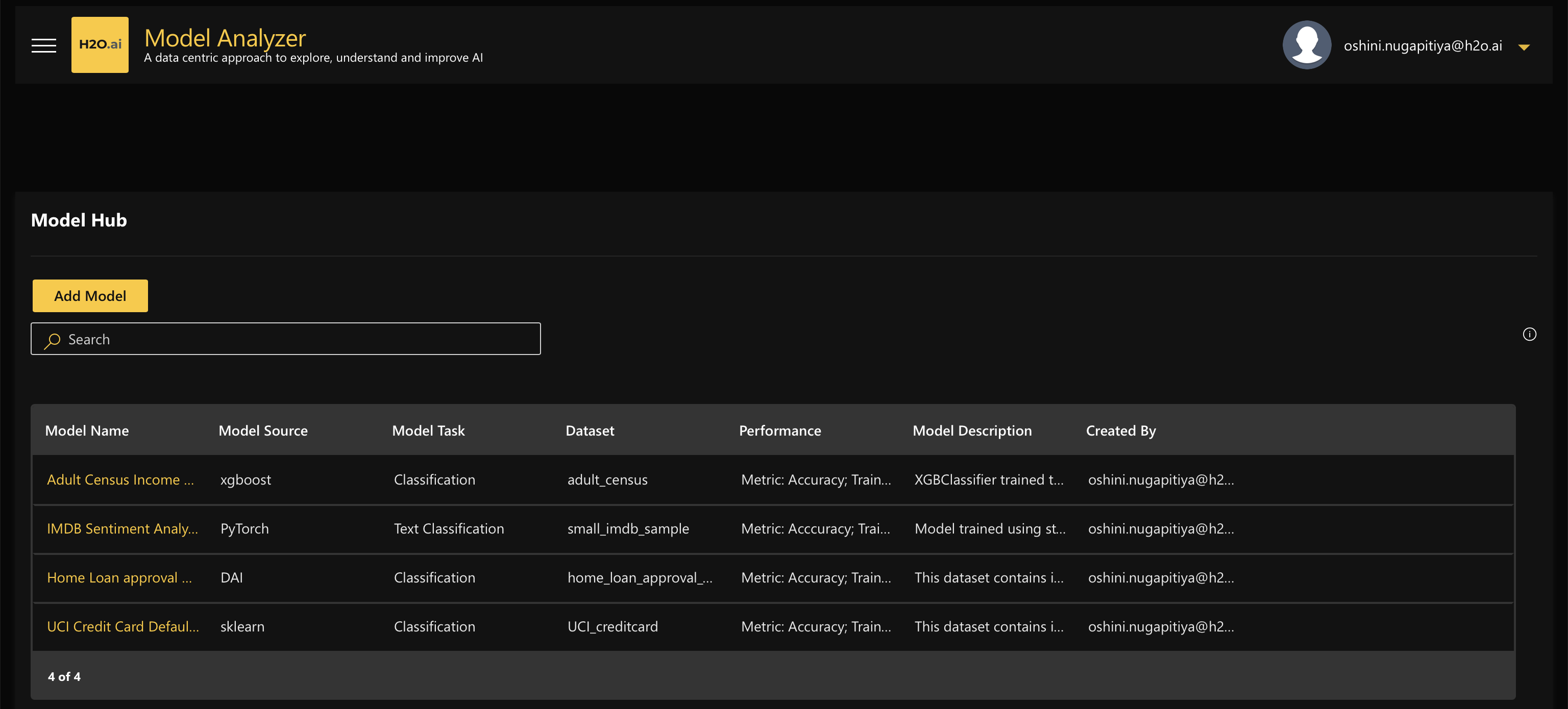
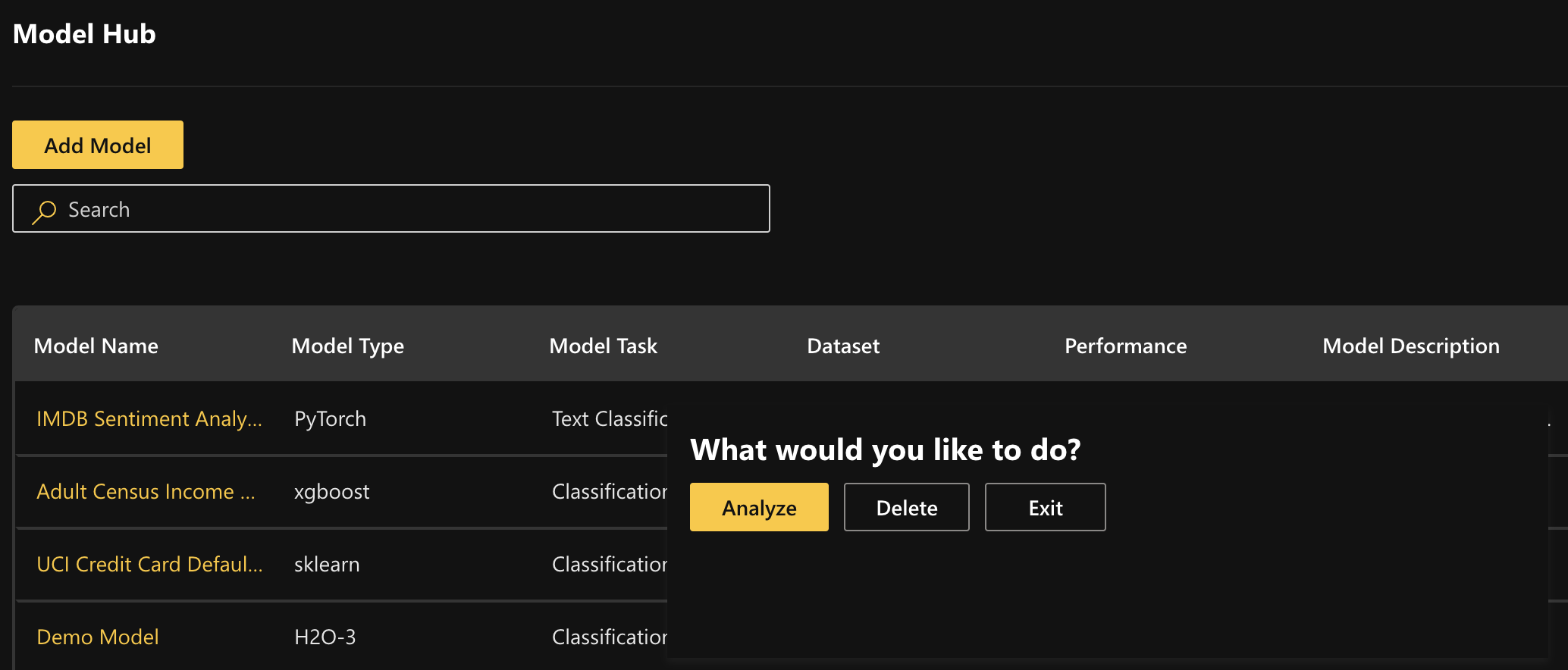
On the H2O Model Analyzer home page, click “Add Model”:
-
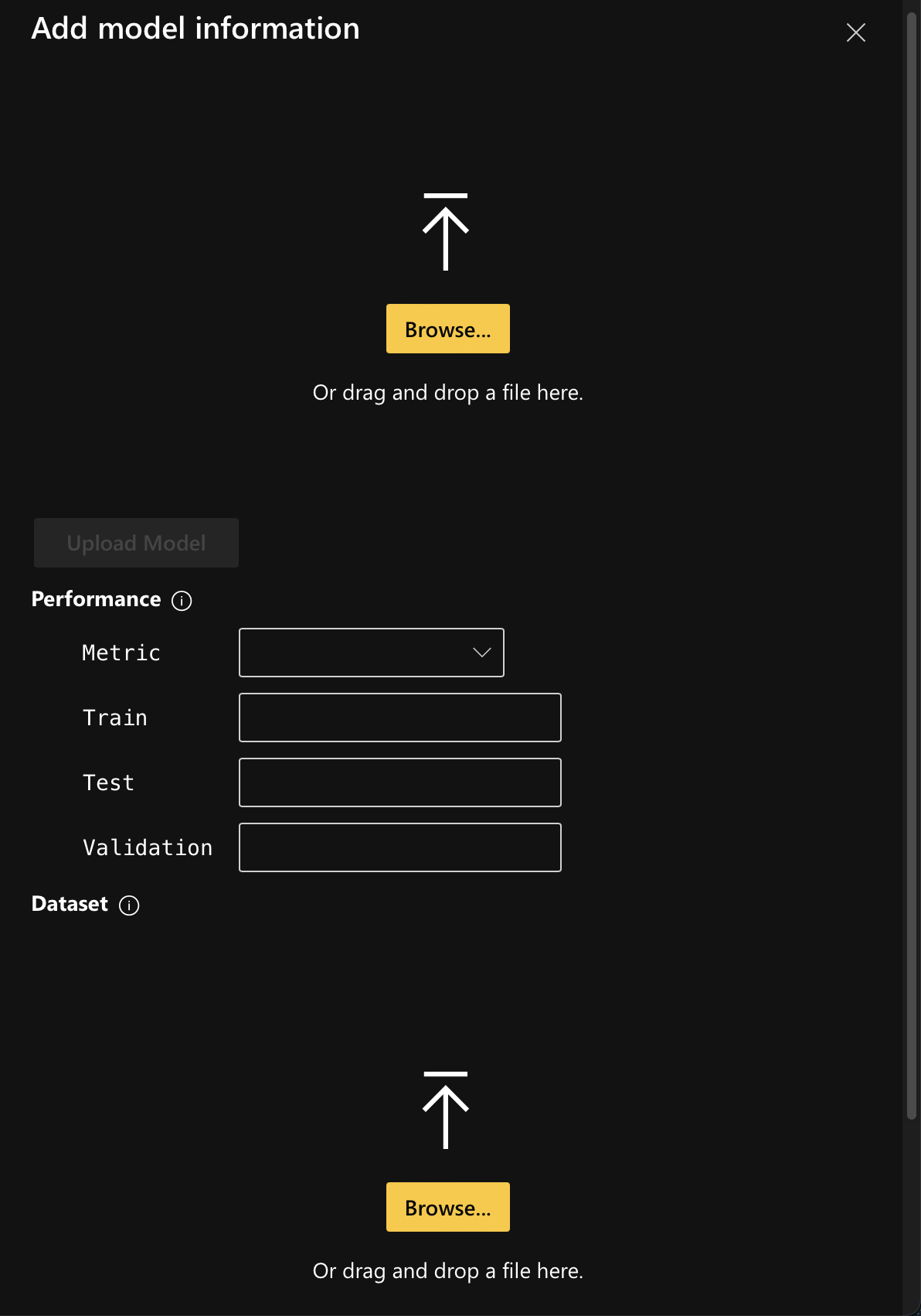
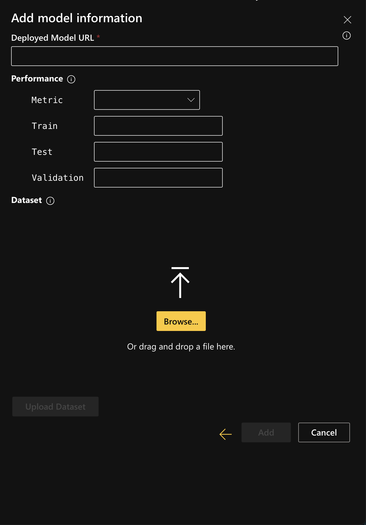
Add model information:

If you select the model type as In-memory model, upload the model and the associated dataset from your device.
If you select the model type as a Deployed model, enter the deployed model URL and upload the associated dataset.
-
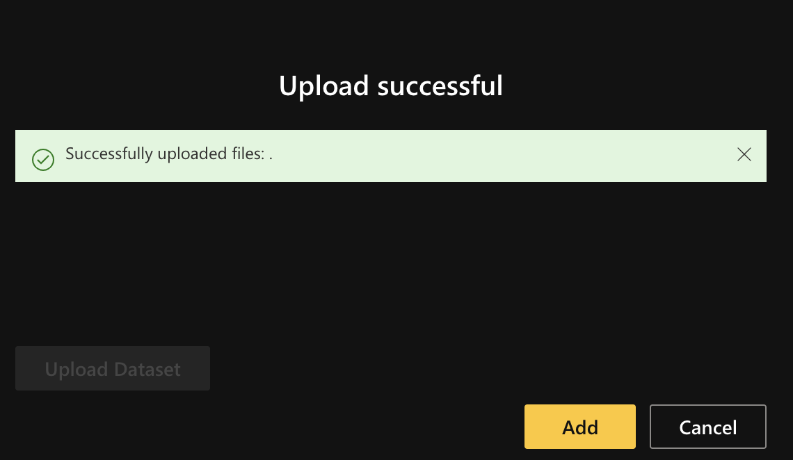
Once the upload is successful, click on "Add" to register a new model:
-
Start analysis by double-clicking on registered model:
-
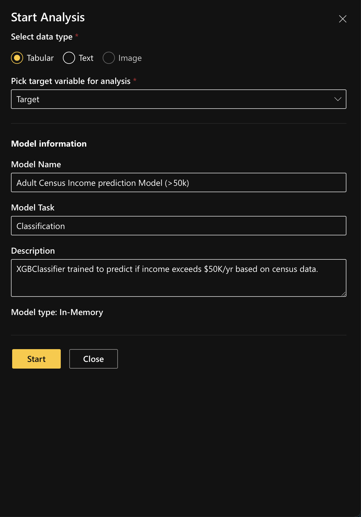
Click “Analyze” and start the analysis by selecting the data type (e.g., Tabular) and picking target variable for analysis:
-
Now you are ready to analyze the model with its associated data:
-
Use Demo Model and Dataset
To make getting familiar with Model Analyzer easier, we have added a few sample models and datasets. You can select one of the following datasets:
-
UCI Credit Card Default Prediction Model - UCI_creditcard
- Model Type: sklearn
- Model Task: Binary Classification
- Dataset: UCI Default Credit Card Clients dataset (UCI_creditcard)
-
IMDB Sentiment Analysis Model
- Model Type: PyTorch
- Model Task: Text Classification
- Dataset: IMDB dataset (small_imdb_sample)
-
Adult Census Income prediction Model (>50k)
- Model Type: xgboost
- Model Task: Binary Classification
- Dataset: UCI Adult Census Income dataset (adult_census)
-
Home Loan approval prediction model
- Model Type: DAI
- Model Task: Binary Classification
- Dataset: Loan Approval Prediction dataset (home_loan_approval_prediction_train)
Step 2: Start analysis
The platform currently supports two ways to analyze a model,
- Select a datapoint of interest for exploration.
- Select multiple datapoints for exploration
Step 2.1.1: Start analysis by selecting a datapoint of interest
To start the discovery and analysis process, you must select a datapoint to initialize the app. You can visualize the data points in the data editor view in one of two ways:
-
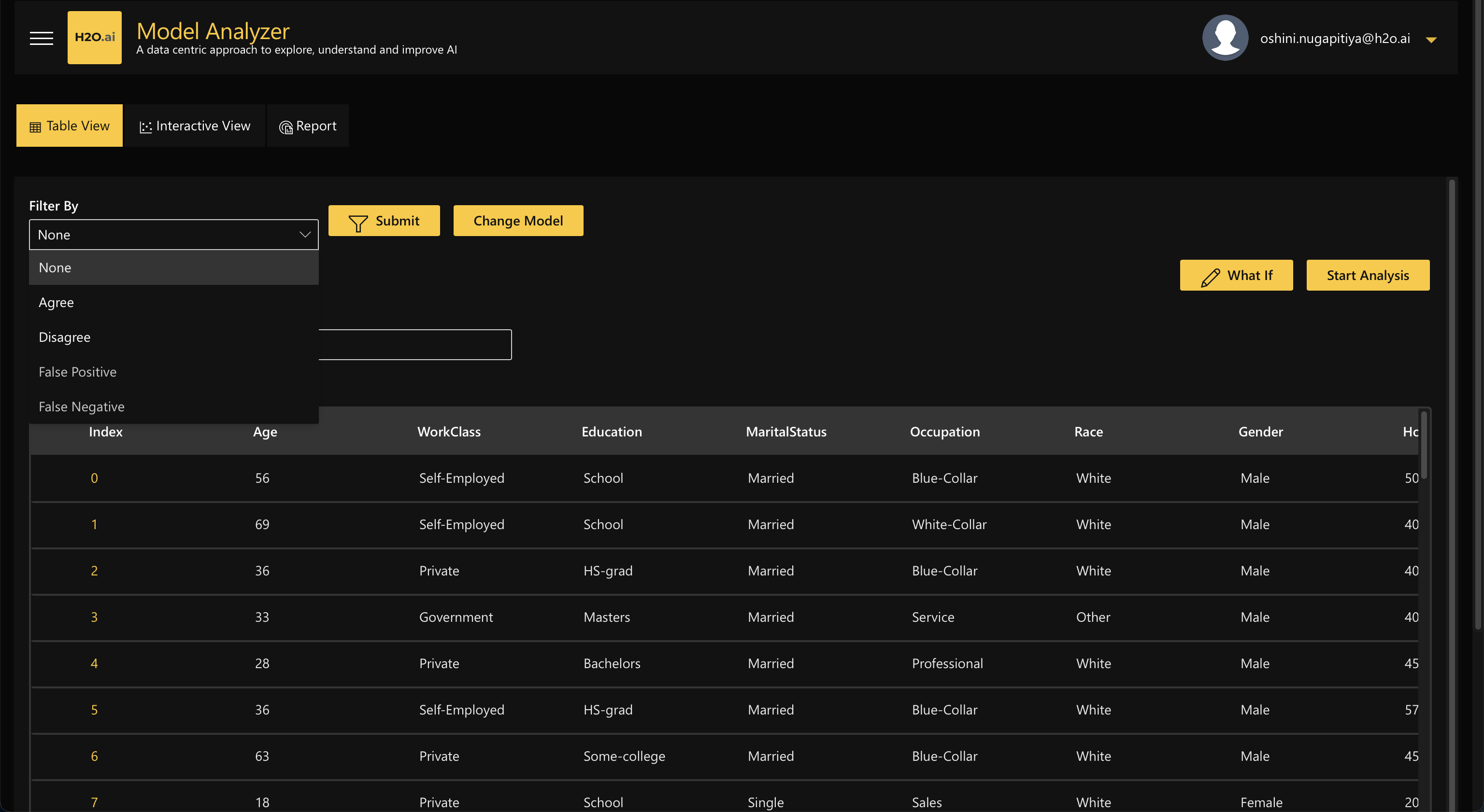
Tabular View: All data points loaded can be seen in a table, along with the target column (if available).
-
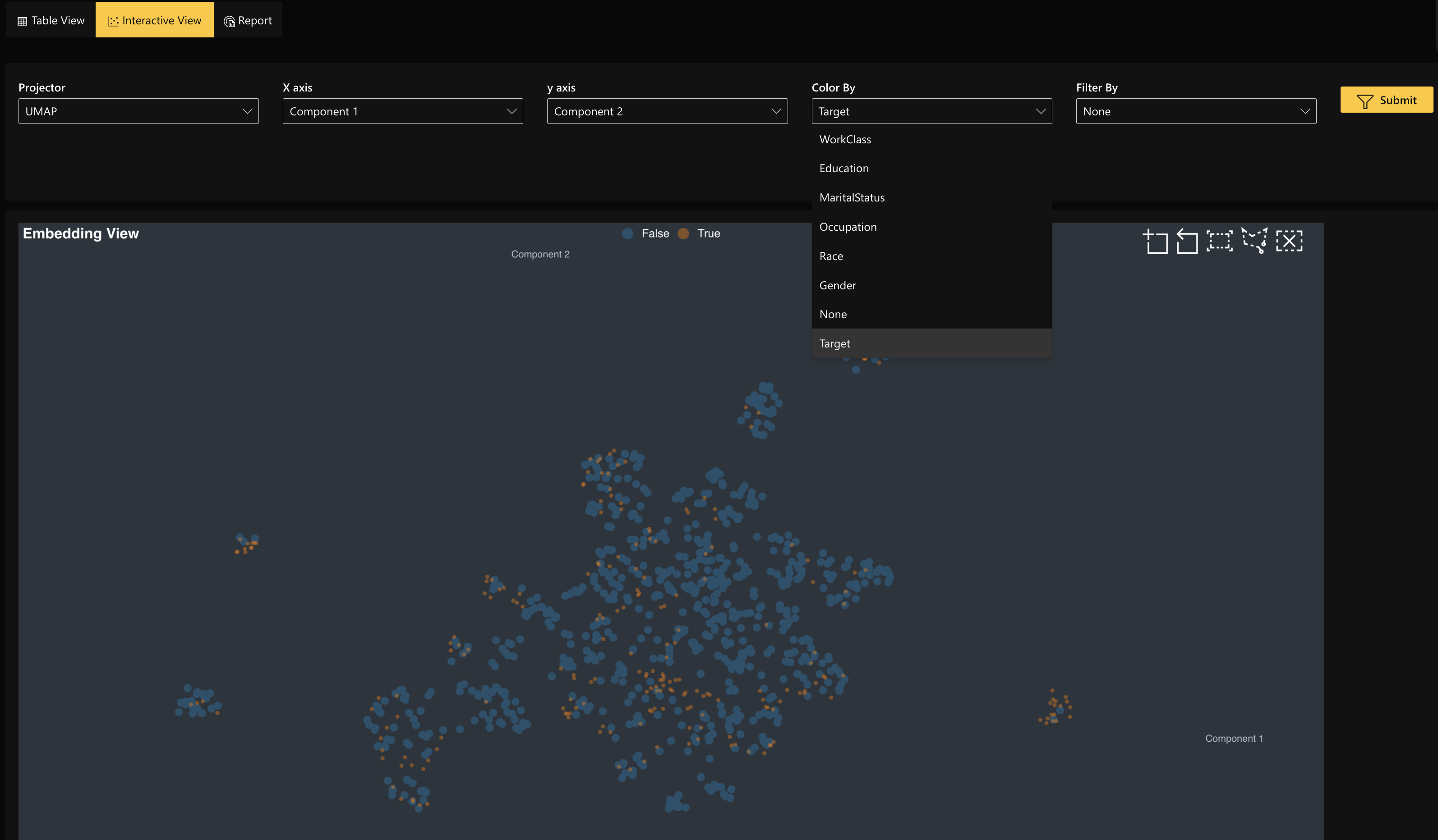
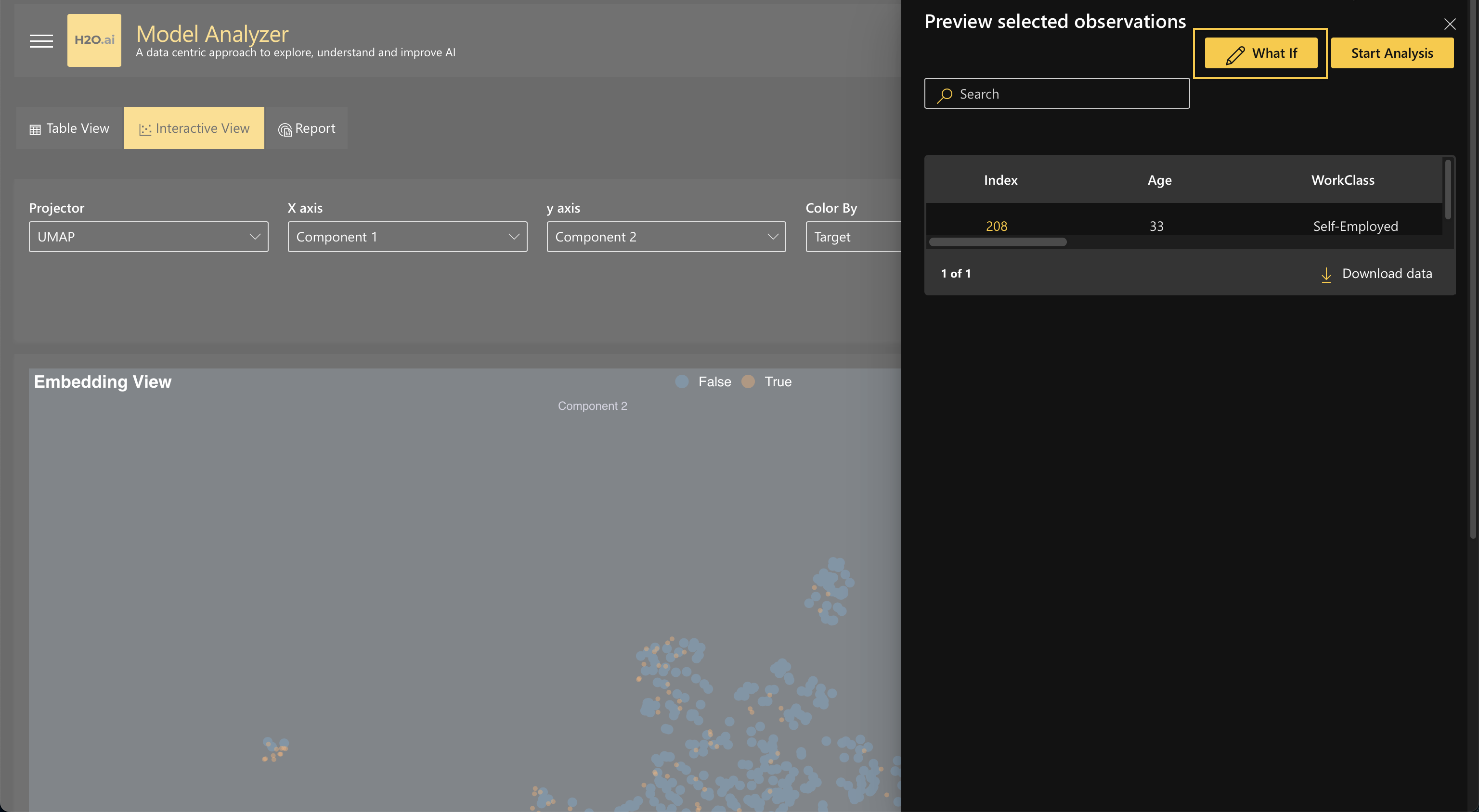
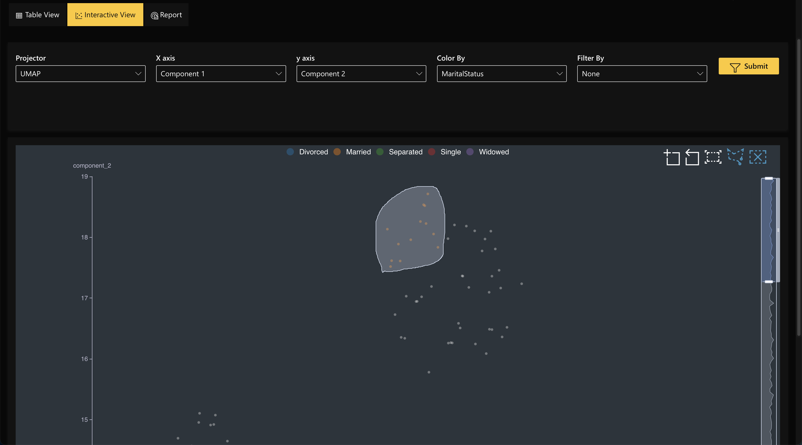
Interactive View: Each point on the chart is a data point. By default, the system projects the data using dimensionality reduction (UMAP), but the user has the ability for further customizations,
- Users can toggle the X and Y axis to visualize the data in different ways
- Users can select different filters to be able to (a) see the data points that agreed (prediction matches ground truth), (b) see the data points that disagreed (prediction does not match ground truth), and (c) see all of the data points.
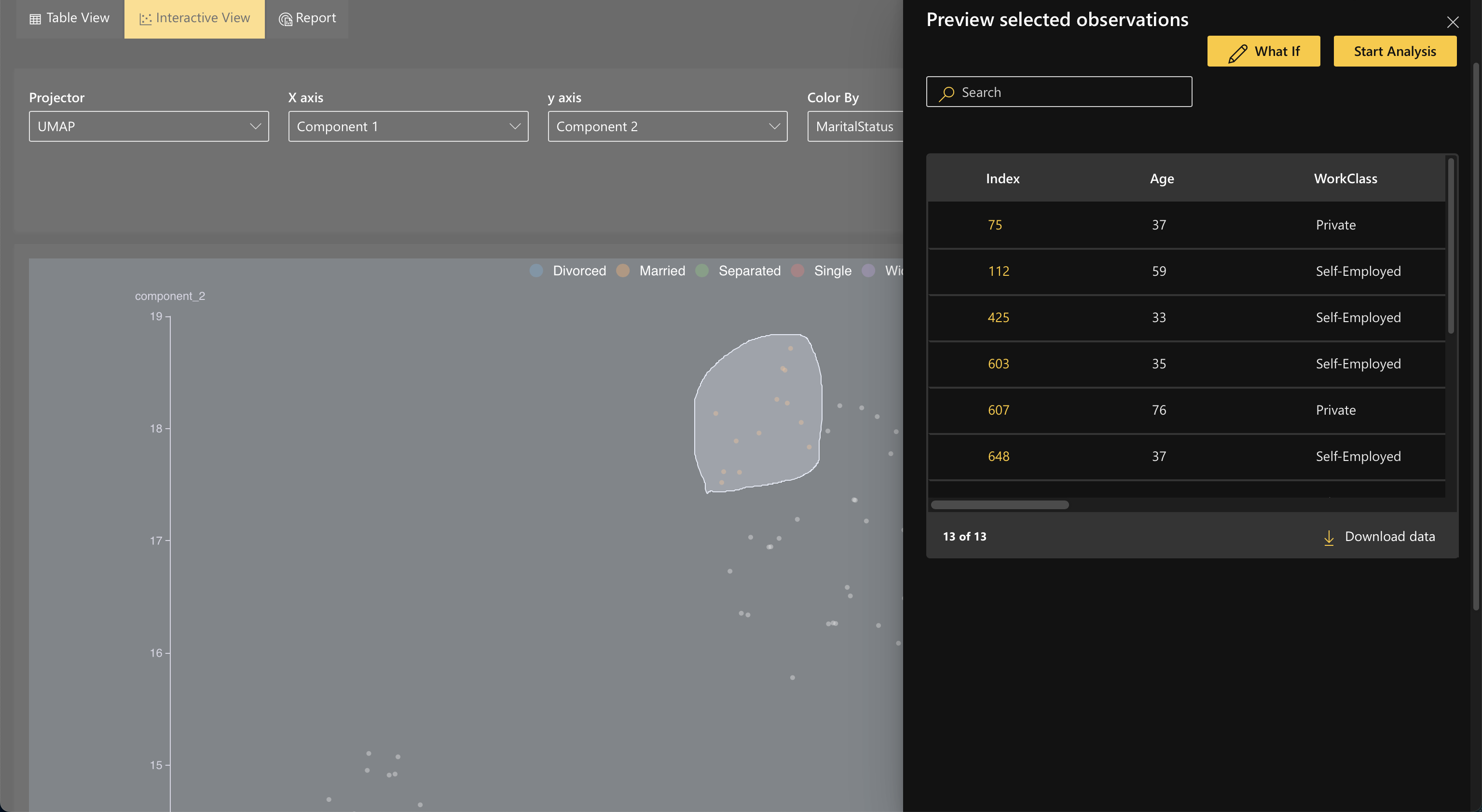
Once you select a data point through either view, click the What if button to open the data editor. This is where your analysis will begin.
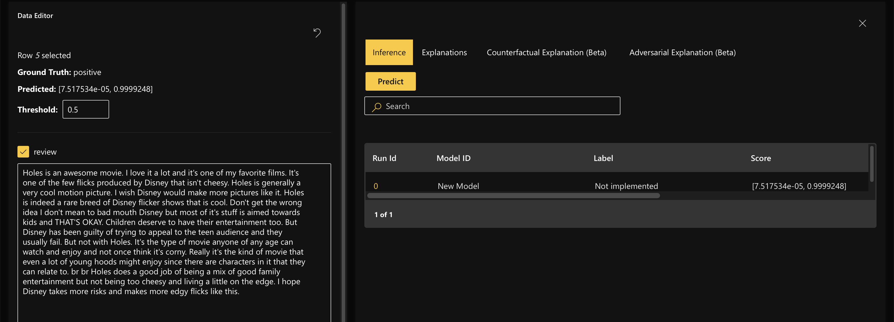
Step 2.1.2: Modify values in Data Editor
In the Data Editor, you are able to simulate scenarios on how the model would behave, given a change in the data input. Once you have changed values in the Data Editor, click on “Predict” to see what the new prediction would be.
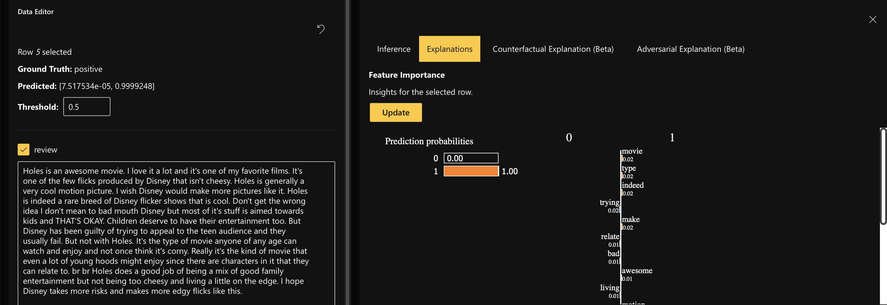
You can also click on the “Explanations” tab to understand local feature importance for the selected datapoint.
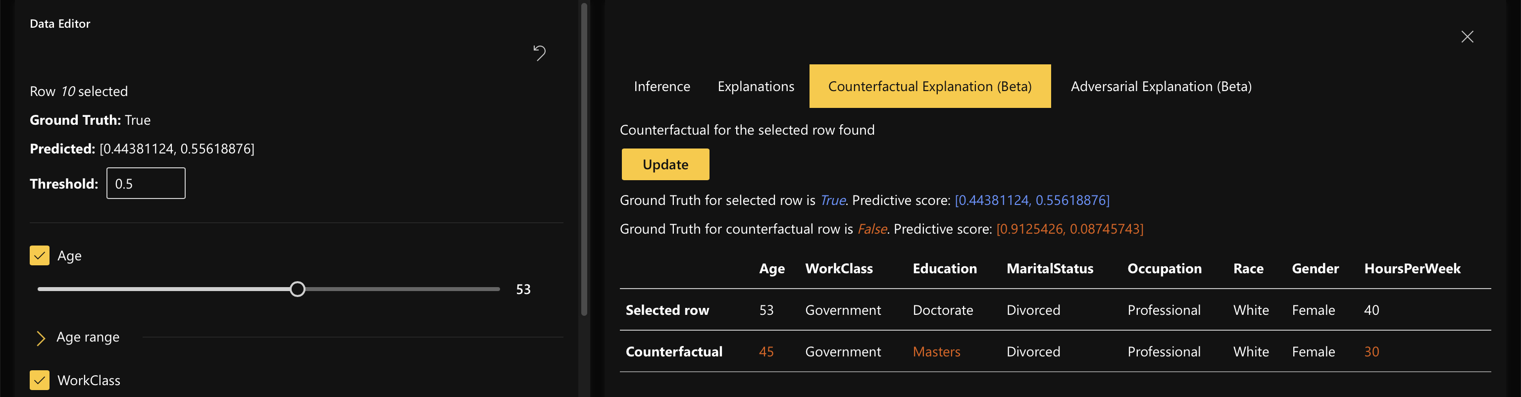
Step 2.1.3: View Counterfactual Explanations and Adversarial Explanations
Counterfactual Explanations
Counterfactual Explanations help you identify the most similar point in your dataset that had a different prediction/outcome from the original data input. This enables you to understand how robust a model is for a data point within your dataset.
For example, if a counterfactual identified is very similar to the original data point and has a different outcome, you would know to retrain the model with similar data points to ensure that the model is robust.
Counterfactual Explanations are not available for the text data type.
You can modify data points from the Data Editor on the left side and click on “Update” to see an updated counterfactual.
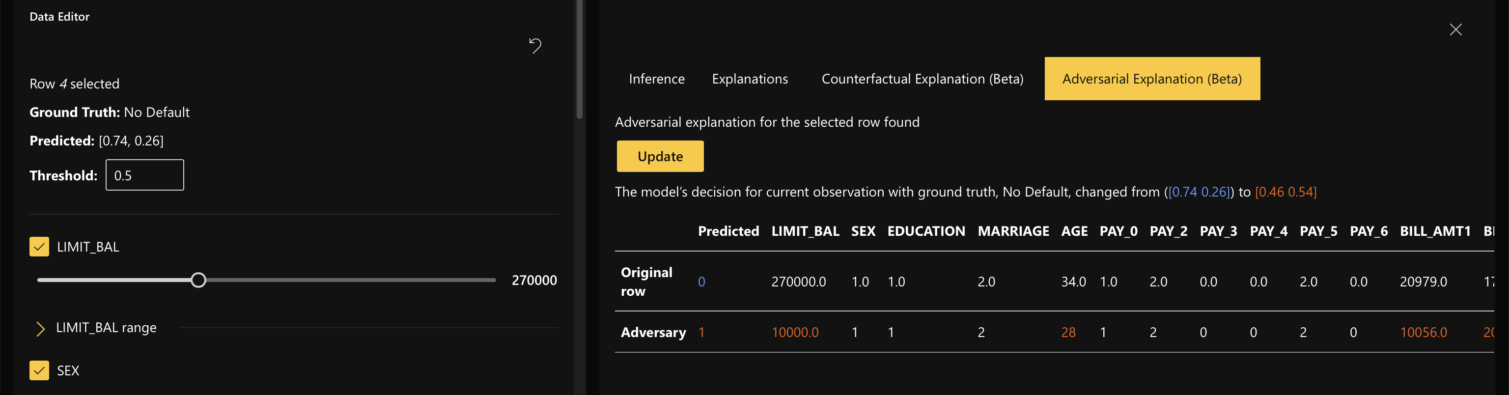
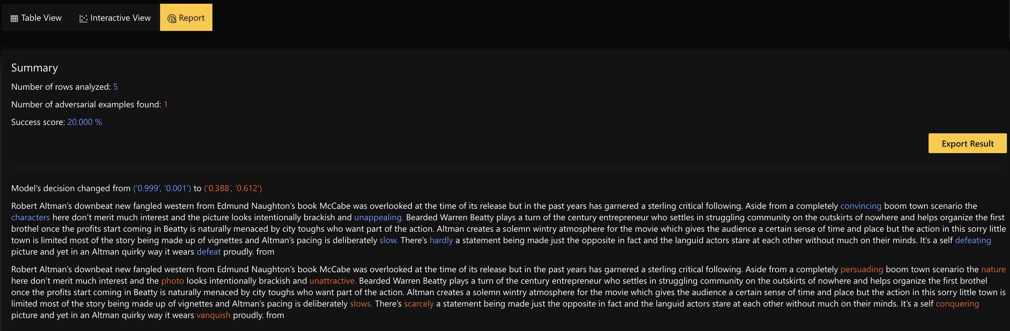
Adversarial Explanations
Adversarial Explanations help you generate a new data point that is most similar to your existing data point, and would have a different prediction/outcome. This enables you to understand the robustness of your model for data points that your model has not seen yet.
In order to generate adversarial explanations, click on the Adversarial Explanation tab and click on “Generate.”

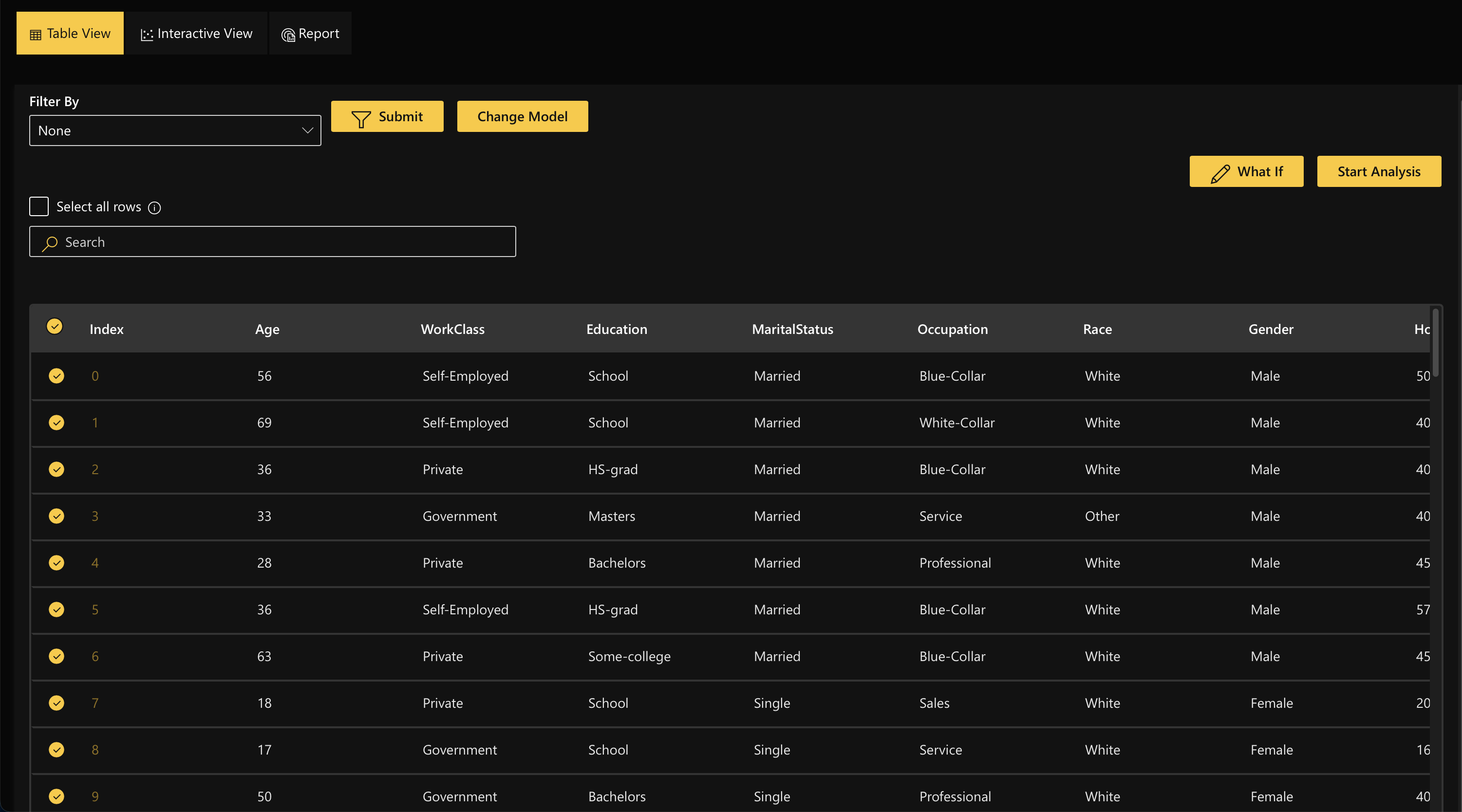
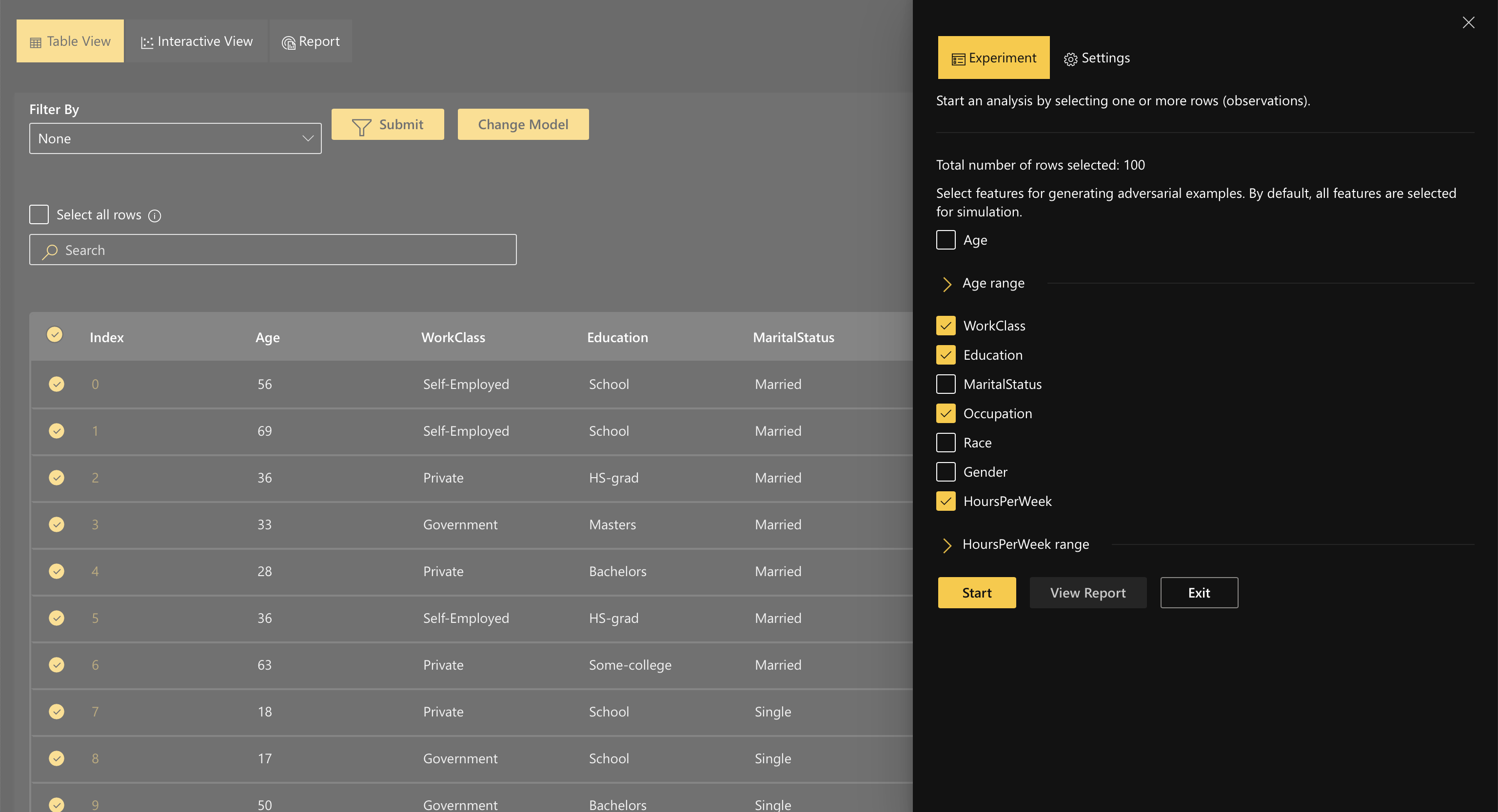
Step 2.2.1: Start analysis by selecting multiple rows
Exploring thousands of observations might get overwhelming and time-consuming to analyze single data points. The platform allows users to select multiple rows and start a job to examine possible adversarial examples.
Step 2.2.2 Table View
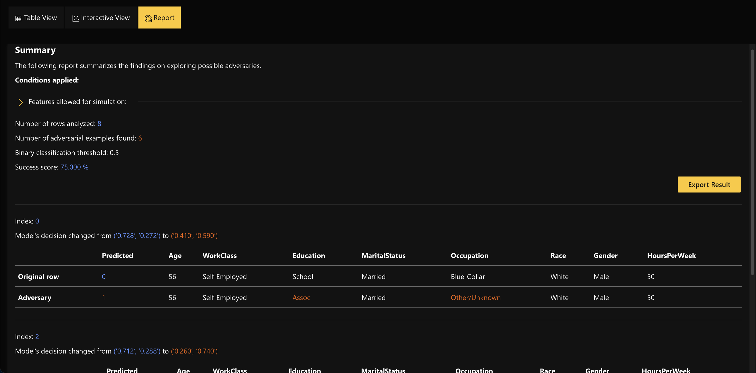
Step 2.2.3 Report View
Once a job is complete users can view the analysis in the report view
Step 2.2.3 Interactive View
Users can discover erroneous points interactively and select cohorts for further analysis
- Submit and view feedback for this page
- Send feedback about H2O Model Analyzer to cloud-feedback@h2o.ai