Experiments¶

Before You Begin¶

This section describes how to run an experiment using the Driverless AI UI. Before you begin, it is best that you understand the available options that you can specify. Note that only a dataset and a target column are required to be specified, but Driverless AI provides a variety of experiment and expert settings that you can use to build your models.

After you have a comfortable working knowledge of these options, proceed to the New Experiments section.

Experiment Settings¶

This section describes the settings that are available when running an experiment.

Dropped Columns¶

Dropped columns are columns that you do not want to be used as predictors in the experiment. Note that Driverless AI will automatically drop ID columns and columns that contain a significant number of unique values (above max_relative_cardinality in the config.toml file or Max. allowed fraction of uniques for integer and categorical cols in Expert settings).

Validation Dataset¶

The validation dataset is used for tuning the modeling pipeline. If provided, the entire training data will be used for training, and validation of the modeling pipeline is performed with only this validation dataset. This is not generally recommended, but can make sense if the data are non-stationary. In such a case, the validation dataset can help to improve the generalization performance on shifting data distributions.

This dataset must have the same number of columns (and column types) as the training dataset. Also note that if provided, the validation set is not sampled down, so it can lead to large memory usage, even if accuracy=1 (which reduces the train size).

Test Dataset¶

The test dataset is used for testing the modeling pipeline and creating test predictions. The test set is never used during training of the modeling pipeline. (Results are the same whether a test set is provided or not.) If a test dataset is provided, then test set predictions will be available at the end of the experiment.

Weight Column¶

Optional: Column that indicates the observation weight (a.k.a. sample or row weight), if applicable. This column must be numeric with values >= 0. Rows with higher weights have higher importance. The weight affects model training through a weighted loss function and affects model scoring through weighted metrics. The weight column is not used when making test set predictions, but a weight column (if specified) is used when computing the test score.

Fold Column¶

Optional: Column to use to create stratification folds during (cross-)validation, if applicable. Must be of integer or categorical type. Rows with the same value in the fold column represent cohorts, and each cohort is assigned to exactly one fold. This can help to build better models when the data is grouped naturally. If left empty, the data is assumed to be i.i.d. (identically and independently distributed). For example, when viewing data for a pneumonia dataset, person_id would be a good Fold Column. This is because the data may include multiple diagnostic snapshots per person, and we want to ensure that the same person’s characteristics show up only in either the training or validation frames, but not in both to avoid data leakage. Note that a fold column cannot be specified if a validation set is used or if a Time Column is specified.

Time Column¶

Optional: Column that provides a time order (time stamps for observations), if applicable. Can improve model performance and model validation accuracy for problems where the target values are auto-correlated with respect to the ordering (per time-series group).

The values in this column must be a datetime format understood by pandas.to_datetime(), like “2017-11-29 00:30:35” or “2017/11/29”, or integer values. If [AUTO] is selected, all string columns are tested for potential date/datetime content and considered as potential time columns. If a time column is found, feature engineering and model validation will respect the causality of time. If [OFF] is selected, no time order is used for modeling and data may be shuffled randomly (any potential temporal causality will be ignored).

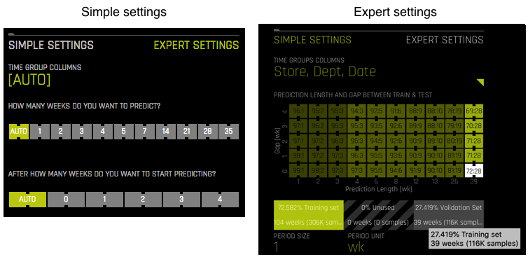
When your data has a date column, then in most cases, specifying [AUTO] for the Time Column will be sufficient. However, if you select a specific date column, then Driverless AI will provide you with an additional side menu. At a minimum, this side menu will allow you to specify the number of weeks you want to predict and, if a test set is provided, after how many weeks do you want to start predicting. These options default to [AUTO]. Or you can select Expert Settings to specify per-group periodicities, such as a time-store group or a time-customer_id group. You can also adjust the period unit, which will in turn change the period size. Available period units include: nanosecond, microsecond, millisecond second, minute, hour, day, week, month, quarter, year.

Notes:

Engineered features will be used for MLI when a time series experiment is built. This is because munged time series features are more useful features for MLI compared to raw time series features.
A Time Column cannot be specified if a Fold Column is specified. This is because both fold and time columns are only used to split training datasets into training/validation, so once you split by time, you cannot also split with the fold column. If a Time Column is specified, then the time group columns play the role of the fold column for time series.
A Time Column cannot be specified if a validation dataset is used.

Refer to Time Series in Driverless AI for more information about time series experiments in Driverless AI and to see a time series example.

Accuracy, Time, and Interpretability Knobs¶

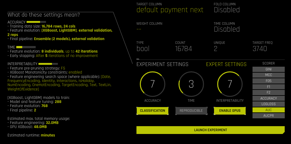
The experiment preview describes what the Accuracy, Time, and Interpretability settings mean for your specific experiment. This preview will autmatically update if any of the knob values change. Following is more detailed information describing how these values affect an experiment.

Accuracy¶

As accuracy increases (as indicated by the tournament_* toml settings), Driverless AI gradually adjusts the method for performing the evolution and ensemble. At low accuracy, Driverless AI varies features and models, but they all compete evenly against each other. At higher accuracy, each independent main model will evolve independently and be part of the final ensemble as an ensemble over different main models. At higher accuracies, Driverless AI will evolve+ensemble feature types like Target Encoding on and off that evolve independently. Finally, at highest accuracies, Driverless AI performs both model and feature tracking and ensembles all those variations.

The following table describes how the Accuracy value affects a Driverless AI experiment.

Accuracy	Max Rows x Cols	Ensemble Level	Target Transformation	Parameter Tuning Level	Num Individuals	Num Folds	Only First Fold Model	Distribution Check
1	100K	0	False	0	Auto	3	True	No
2	1M	0	False	0	Auto	3	True	No
3	50M	0	True	1	Auto	3	True	No
4	100M	0	True	1	Auto	3-4	True	No
5	200M	1	True	1	Auto	3-4	True	Yes
6	500M	2	True	1	Auto	3-5	True	Yes
7	750M	<=3	True	2	Auto	3-10	Auto	Yes
8	1B	<=3	True	2	Auto	4-10	Auto	Yes
9	2B	<=3	True	3	Auto	4-10	Auto	Yes
10	10B	<=4	True	3	Auto	4-10	Auto	Yes

Note: A check for a shift in the distribution between train and test is done for accuracy >= 5.

The list below includes more information about the parameters that are used when calculating accuracy.

Max Rows x Cols: The maximum number of rows x colums to use in model training
- For classification, stratified random row sampling is performed (by target)
- For regression, random row sampling is performed
Ensemble Level: The level of ensembling done for the final model (if no time column is selected)
- 0: single model
- 1: 1x 4-fold models ensembled together
- 2: 2x 5-fold models ensembled together
- 3: 5x 5-fold models ensembled together
- 4: 8x 5-fold models ensembled together
- If ensemble level > 0, then the final model score shows an error estimate that includes the data generalization error (standard deviation of scores over folds) and the error in the estimate of the score (bootstrap score’s standard deviation with sample size same as data size).
- For accuracy >= 8, the estimate of the error in the validation score reduces, and the error in the score is dominated by the data generalization error.
- The estimate of the error in the test score is estimated by the maximum of the bootstrap with sample size equal to the test set size and the validation score’s error.
Target Transformation: Try target transformations and choose the transformation(s) that have the best score(s).

Possible transformations: identity, unit_box, log, square, square root, double square root, inverse, Anscombe, logit, sigmoid
Parameter Tuning Level: The level of parameter tuning done
- 0: no parameter tuning
- 1: 8 different parameter settings
- 2: 16 different parameter settings
- 3: 32 different parameter settings
- 4: 64 different parameter settings
- Optimal model parameters are chosen based on a combination of the model’s accuracy, training speed, and complexity.
Num Individuals: The number of individuals in the population for the genetic algorithms
- Each individual is a gene. The more genes, the more combinations of features are tried.
- The number of individuals is automatically determined and can depend on the number of GPUs. Typical values are between 4 and 16.
Num Folds: The number of internal validation splits done for each pipeline
- If the problem is a classification problem, then stratified folds are created.
Only First Fold Model: Whether to only use the first fold split for internal validation to save time
- Example: Setting Num Folds to 3 and Only First Fold Model = True means you are splitting the data into 67% training and 33% validation.
- If “Only First Fold Model” is False, then errors on the score shown during feature engineering include the data generalization error (standard deviation of scores over folds) and the error in the estimate of the score (bootstrap score’s standard deviation with a sample size the same as the data size).
- If “Only First Fold Model” is True, then errors on the score shown during feature engineering include only the error in the estimate of the score (bootstrap score’s standard deviation with a sample size same as the data size).
- For accuracy >= 8, the estimate of the error in the score reduces, and the error in the score is dominated by the data generalization error. This provides the most accurate generalization error.
Early Stopping Rounds: Time-based means based upon the Time table below.
Distribution Check: Checks whether validation or test data are drawn from the same distribution as the training data. Note that this is purely informative to the user. Driverless AI does not take information from the test set into consideration during training.
Strategy: Feature selection strategy (to prune-away features that do not clearly give improvement to model score). Feature selection is triggered by interpretability. Strategy = “FS” if interpretability >= 6; otherwise strategy is None.

Time¶

This specifies the relative time for completing the experiment (i.e., higher settings take longer). Early stopping will take place if the experiment doesn’t improve the score for the specified amount of iterations.

Time	Iterations	Early Stopping Rounds
1	1-5	None
2	10	5
3	30	5
4	40	5
5	50	10
6	100	10
7	150	15
8	200	20
9	300	30
10	500	50

Note: See the Accuracy table for cases when not based upon time.

Interpretability¶

In the following tables, Ensemble Level is the level of ensembling done for the final model (if no time column is selected).

0: single model

1: 1x 4-fold models ensembled together

2: 2x 5-fold models ensembled together

3: 5x 5-fold models ensembled together

If Monotonicity Constraints are enabled, the model will satisfy knowledge about monotonicity in the data and monotone relationships between the predictors and the target variable. For example, in house price prediction, the house price should increase with lot size and number of rooms, and should decrease with crime rate in the area. If enabled, Driverless AI will automatically determine if monotonicity is present and enforce it in its modeling pipelines. Depending on the correlation, Driverless AI will assign positive, negative, or no monotonicity constraints. Monotonicity is enforced if the absolute correlation is greater than 0.1. All other predictors will not have monotonicity enforced.

Interpretability	Ensemble Level	Monotonicity Constraints
<= 5	<= 3	Disabled
>= 6	<= 2	Disabled
>= 7	<= 2	Enabled
>= 8	<= 1	Enabled
10	0	Enabled

Interpretability	Transformers**
<= 5	All
0-5	Interpretability#5 - [TruncSvdNum, ClusterDist]
0-6	Interpretability#6 - [ClusterTE, ClusterID, IsolationForestAnomaly]
0-7	Interpretability#7 - [NumToCatTE]
0-8	Interpretability#8 - [NumCatTE, NumToCatWoE]
0-9	Interpretability#9 - [BulkInteractions, WeightOfEvidence, CvCatNumEncode, NumToCatWeightOfEvidenceMonotonic]
0-10	Interpretability#10 - [CVTargetEncodeFit, CVCatNumericEncodeF, Frequent]

** Interpretability# - [lost transformers] explains which transformers are lost by going up by 1 to that interpretability.

** Exception - NumToCatWeightOfEvidenceMonotonic removed for interpretability<=6.

** For interpretability <= 10, i.e. only [Filter for numeric, Frequent for categorical, DateTime for Date+Time, Date for dates, and Text for text]

Target Transformers:

For regression, applied on target before any other transformations.

Interpretability	Target Transformer
<=10	TargetTransformer_identity
<=10	TargetTransformer_unit_box
<=10	TargetTransformer_log
<= 9	TargetTransformer_square
<= 9	TargetTransformer_sqrt
<= 8	TargetTransformer_double_sqrt
<= 6	TargetTransformer_logit
<= 6	TargetTransformer_sigmoid
<= 5	TargetTransformer_Anscombe
<= 4	TargetTransformer_inverse

Date Types Detected:
- categorical
- date
- datetime
- numeric
- text

Transformers used on raw features to generate new features:

Interpretability	Transformer
<=10	Filter
<=10	DateTime
<=10	Date
<=10	Text
<=10	TextLin
<=10	CvTargetEncodeMulti
<=10	CvTargetEncodeSingle
<=9	CvCatNumEncode
<=9	WeightOfEvidence
<=9 and >=7	NumToCatWeightOfEvidenceMonotonic
<=9	BulkInteractions
<=8	NumToCatWeightOfEvidence
<=8	NumCatTargetEncodeMulti
<=8	NumCatTargetEncodeSingle
<=7	Frequent
<=7	NumToCatTargetEncodeMulti
<=7	NumToCatTargetEncodeSingle
<=6	ClusterIDTargetEncodeMulti
<=6	ClusterIDTargetEncodeSingle
<=5	TruncSvdNum
<=5	ClusterDist

** Default N-way interactions are up to 8-way except:

BulkInteractions are always 2-way.
Interactions are minimal-way (e.g. 1-way for CvTargetEncode) if interpretability=10.

Feature importance threshold below which features are removed

Interpretability	Threshold
10	config.toml varimp_threshold_at_interpretability_10
9	varimp_threshold_at_interpretability_10/5.0
8	varimp_threshold_at_interpretability_10/7.0
7	varimp_threshold_at_interpretability_10/10.0
6	varimp_threshold_at_interpretability_10/20.0
5	varimp_threshold_at_interpretability_10/30.0
4	varimp_threshold_at_interpretability_10/50.0
3	varimp_threshold_at_interpretability_10/500.0
2	varimp_threshold_at_interpretability_10/5000.0
1	1E-30

** Also used for strategy=FS dropping of features, but the threshold is the above value multiplied by config.varimp_fspermute_factor.

Base model used for scoring features and building final model

Interpretability	Allowed Base Model
10	Only GLM if glm_enable_more==True or glm_enable_exlcusive=True, GBM+GLM if glm_enable==True, else only GBM
9	GBM unless glm_enable_exlcusive=True, GBM+GLM if glm_enable_more==True
8	GBM unless glm_enable_exlcusive=True, GBM+GLM if glm_enable_more==True
7	GBM unless glm_enable_exlcusive=True, GBM+GLM if glm_enable_more==True
6	GBM unless glm_enable_exlcusive=True, GBM+GLM if glm_enable_more==True
5	GBM unless glm_enable_exlcusive=True
4	GBM unless glm_enable_exlcusive=True
3	GBM unless glm_enable_exlcusive=True
2	GBM unless glm_enable_exlcusive=True
1	GBM unless glm_enable_exlcusive=True

** When mixing GBM and GLM in parameter tuning, the search space is split 50%/50% between GBM and GLM.

Classification, Reproducible, and Enable GPUs Buttons¶

Classification or Regression button. Driverless AI automatically determines the problem type based on the response column. Though not recommended, you can override this setting by clicking this button.
Reproducible: This button allows you to build an experiment with a random seed and get reproducible results. If this is disabled (default), then results will vary between runs.
Enable GPUs: Specify whether to enable GPUs. (Note that this option is ignored on CPU-only systems.)

Expert Settings¶

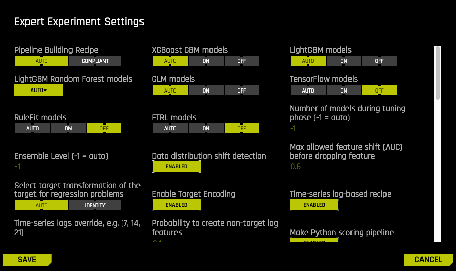
This section describes the Expert Settings options that are available when starting an experiment. Note that the default values for these options are derived from the environment variables in the config.toml file. Refer to the Sample Config.toml File section for more information about each of these options.

Note that by default the feature brain pulls in any better model regardless of the features even if the new model disabled those features. For full control over features pulled in via changes in these Expert Settings, users should set the Feature Brain Level option to 0.

Pipeline Building Recipe¶

Specify the Pipeline Building recipe type. Auto (default) specifies that all models and features are automatically determined by experiment settings, config.toml settings, and the feature engineering effort. Compliant is similar to Auto except for the following:

Interpretability is forced to be 10.
Only use GLM or RuleFit.
Does not convert any numerics to categoricals except via one-hot encoding.
Doesn’t use any ensemble.
No feature brain is used.
Interaction depth is set to 1.
Target transformer is forced to be identity for regression.
Doesn’t use distribution shift between train, valid, and test to drop features.

XGBoost GBM Models¶

This option allows you to specify whether to build XGBoost models as part of the experiment (for both the feature engineering part and the final model). XGBoost is a type of gradient boosting method that has been widely successful in recent years due to its good regularization techniques and high accuracy. This is set to Auto by default.

LightGBM Models¶

This option allows you to specify whether to build LightGBM models as part of the experiment. LightGBM Models are the default models. This is set to Auto by default.

LightGBM Random Forest Models¶

Select auto (default), on, off, or only from this dropdown to specify whether to include LightGBM Random Forest models as part of the experiment.

GLM Models¶

This option allows you to specify whether to build GLM models (generalized linear models) as part of the experiment (usually only for the final model unless it’s used exclusively). GLMs are very interpretable models with one coefficient per feature, an intercept term and a link function. This is set to Auto by default.

TensorFlow Models¶

This option allows you to specify whether to build TensorFlow models as part of the experiment (usually only for text features engineering and for the final model unless it’s used exlusively). Enable this option for NLP experiments. This is disabled by default.

TensorFlow models are not supported by MOJOs (only Python scoring pipelines are supported).

RuleFit Models¶

This option allows you to specify whether to build RuleFit models as part of the experiment. This is disabled by default. Note that MOJOs are not supported (only Python scoring pipelines). Also note that multiclass classification is not supported for RuleFit models. Rules are stored as text files in the experiment directory.

FTRL Models¶

This option allows you to specify whether to build Follow the Regularized Leader (FTRL) models as part of the experiment. This is disabled by default. Note that MOJOs are not supported (only Python scoring pipelines). FTRL supports binomial and multinomial classification for categorical targets, as well as regression for continuous targets.

Number of Models During Tuning Phase¶

Specify the number of models to tune during pre-evolution phase. Specify a lower value to avoid excessive tuning, or specify a higher to perform enhanced tuning. This value defaults to -1 (auto).

Ensemble Level¶

Specify one of the following ensemble levels:

-1 = auto, based upon ensemble_accuracy_switch, accuracy, size of data, etc. (Default)
0 = No ensemble, only final single model on validated iteration/tree count. Note that predicted probabilities will not be available. (Refer to the following FAQ.)
1 = 1 model, multiple ensemble folds (cross-validation)
2 = 2 models, multiple ensemble folds (cross-validation)
3 = 3 models, multiple ensemble folds (cross-validation)
4 = 4 models, multiple ensemble folds (cross-validation)

Data Distribution Shift Detection¶

Specify whether Driverless AI should detect data distribution shifts between train/valid/test datasets (if provided). This information is only presented to the user and not acted upon. This is enabled by default.

Max Allowed Feature Shift (AUC) Before Dropping Feature¶

Specify the maximum allowed AUC value for a feature before dropping the feature.

When train and test differ (or train/valid or valid/test) in terms of distribution of data, then there can be a model built that tells you for each row whether the row is in train or test. That model includes an AUC value. If the AUC is above this specified threshold, then Driverless AI will consider it a strong enough shift to drop features that are shifted.

This value defaults to 0.6.

Select Target Transformation of the Target for Regression Problems¶

Specify whether to automatically select target transformation for regression problems. Selecting Identity disables any transformation. This value defaults to Auto.

Enable Target Encoding¶

Specify whether to use Target Encoding when building the model. Target encoding is the process of replacing a categorical value with the mean of the target variable. This is enabled by default.

Time Series Lag-Based Recipe¶

This recipe specifies whether to include Time Series lag features when training a model with a provided (or autodetected) time column. Lag features are the primary automatically generated time series features and represent a variable’s past values. At a given sample with time stamp \(t\), features at some time difference \(T\) (lag) in the past are considered. For example if the sales today are 300, and sales of yesterday are 250, then the lag of one day for sales is 250. Lags can be created on any feature as well as on the target. Lagging variables are important in time series because knowing what happened in different time periods in the past can greatly facilitate predictions for the future. This is enabled by default. More information about time series lag is available in the Time Series Use Case: Sales Forecasting section.

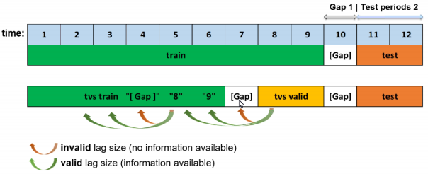
Time Series Lags Override¶

Specify a lag override value such as 7, 14, 21, etc.

Probability to Create Non-Target Lag Features¶

Lags can be created on any feature as well as on the target. Specify a probability value for creating non-target lag features. This value defaults to 0.1.

Make Python Scoring Pipeline¶

Specify whether to automatically build a Python Scoring Pipeline for the experiment. If enabled, then when the experiment is completed, the Python Scoring Pipeline can be immediately downloaded. If disabled, the Python Scoring Pipeline will have to be built separately after the experiment is complete. This is enabled by default.

Make MOJO Scoring Pipeline¶

Specify whether to automatically build a MOJO (Java) Scoring Pipeline for the experiment. If enabled, then when the experiment is completed, the MOJO Scoring Pipeline can be immediately downloaded. If disabled, the MOJO Scoring Pipeline will have to be built separately after the experiment is complete. This is disabled by default.

Max Number of Rules for RuleFit¶

Specify the maximum number of rules to be used for RuleFit models. This defaults to -1, which specifies to use all rules.

Feature Brain Level¶

H2O.ai Brain enables caching and smart re-use (checkpointing) of prior models to generate features for new models. Use this option to specify the brain caching level.

-1: Don’t use any brain cache.
0: Don’t use any brain cache but still write to cache.
1: Smart checkpoint if an old experiment_id is passed in (for example, via running “resume one like this” in the GUI).
2: Smart checkpoint if the experiment matches all column names, column types, classes, class labels, and time series options identically. (Default)
3: Smart checkpoint like level #1, but for the entire population. Tune only if the brain population is of insufficient size.
4: Smart checkpoint like level #2, but for the entire population. Tune only if the brain population is of insufficient size.
5: Smart checkpoint like level #4, but will scan over the entire brain cache of populations (starting from resumed experiment if chosen) in order to get the best scored individuals.

When enabled, the directory where the H2O.ai Brain meta model files are stored is H2O.ai_brain. In addition, the default maximum brain size is 20GB. Both the directory and the maximum size can be changed in the config.toml file.

Quantile-Based Imbalanced Sampling (binary)¶

Specify whether to enable the quantile-based sampling method for imbalanced binary classification. This is disabled by default.(Note: Only applicable if the class ratio is above the imbalanced ratio undersampling threshold.) When enabled, model on data is used to create deciles of predictions, and then each decile is sampled from uniformly.

The idea behind quantile-based imbalanced sampling is that we do not want to just randomly down sample the majority class; instead we want to get an interesting representation of the majority class.

Here are the steps used to perform quantile-based imbalanced sampling:

Train an initial model.
Use the model from Step 1 to score each record in the majority class.
Bin the majority class records based on their prediction.
Randomly sample records from each bin.

If our use case was fraud, then quantile-based imbalanced sampling would sample not-fraud records based on the prediction of an initial model. This ensures that we have an even distribution of records that are easy to classify as not-fraud (low prediction bins) and records that are harder to classify as not-fraud (high prediction bins).

Generate Holiday Features¶

For time-series experiments, enable this option to generate holiday features for the experiment. This is enabled by default.

Random Seed¶

Specify a random seed for the experiment. When a seed is defined and the reproducible button is enabled (not by default), the algorithm will behave deterministically.

Force 64-bit Precision¶

Specify whether to enable 64-bit data and transformer precision. This option is disabled by default, as Driverless AI uses 32-bit floats.

This setting shouldn’t matter unless your data value exceeds 1E38 or if you need to resolve more than 1 part in 10 million. If your data has larger numbers than the above, then you may encounter a Best score is not finite: %f" % best_score\nAssertionError: Best score is not finite: inf\n'} error. This can be resolved by using data_precision="float64" and transformer_precision="float64" in config.toml or by enabling this option.

Min Number of Rows Needed to Run an Experiment¶

Specify the minimum number of rows that a dataset must contain in order to run an experiment. This value defaults to 100.

Max Number of Original Features Used¶

Specify the maximum number of features you want to be selected in an experiment. This value defaults to 10000.

Max Number of Engineered Features¶

Specify the maximum number of features to include in the final model’s feature engineering pipeline. If -1 is specified (default), then Driverless AI will automatically determine the number of features.

Max Number of Rows times the Number of Columns for Feature Evolution Data Splits¶

Specify the maximum number of rows allowed for feature evolution data splits (not for the final pipeline). This value defaults to 100,000,000.

Feature Engineering Effort (0..10)¶

Specify a value from 0 to 10 for the Driverless AI feature engineering effort. Higher values generally lead to more time (and memory) spent in feature engineering. This value defaults to 5.

0: Keep only numeric features. Only model tuning during evolution.
1: Keep only numeric features and frequency-encoded categoricals. Only model tuning during evolution.
2: Similar to 1 but instead just no Text features. Some feature tuning before evolution.
3: Similar to 5 but only tuning during evolution. Mixed tuning of features and model parameters.
4: Similar to 5, but slightly more focused on model tuning.
5: Balanced feature-model tuning. (Default)
6-7: Similar to 5 but slightly more focused on feature engineering.
8: Similar to 6-7 but even more focused on feature engineering with high feature generation rate and no feature dropping even if high interpretability.
9-10: Similar to 8 but no model tuning during feature evolution.

Max Feature Interaction Depth¶

Specify the maximum number of features to be used for interaction features like grouping for target encoding, weight of evidence and other likelihood estimates.

Exploring feature interactions can be important in gaining better predictive performance. The interaction can take multiple forms (i.e. feature1 + feature2 or feature1 * feature2 + … featureN). Although certain machine learning algorithms (like tree-based methods) can do well in capturing these interactions as part of their training process, still generating them may help them (or other algorithms) yield better performance.

The depth of the interaction level (as in “up to” how many features may be combined at once to create one single feature) can be specified to control the complexity of the feature engineering process. Higher values might be able to make more predictive models at the expense of time. This value defaults to 8.

Max Allowed Fraction of Uniques for Integer and Categorical Cols¶

Specify the maximum fraction of unique values for integer and categorical columns. If the column has a larger fraction of unique values than that, it will be considered an ID column and ignored. This value defaults to 0.95.

Threshold for String Columns to be Treated as Text¶

Specify the threshold value (from 0 to 1) for string columns to be treated as text (0.0 - text; 1.0 - string). This value defaults to 0.3.

Max TensorFlow Epochs¶

When building TensorFlow models, specify the maximum number of epochs to train models with (it might stop earlier). This value defaults to 100. This option is ignored if TensorFlow models is disabled.

Enable Word-Based CNN TensorFlow Models for NLP¶

Specify whether to use Word-based CNN TensorFlow models for NLP. This option is ignored if TensorFlow is disabled. This is disabled by default.

Enable Word-Based BiGRU TensorFlow Models for NLP¶

Specify whether to use Word-based BiGRU TensorFlow models for NLP. This option is ignored if TensorFlow is disabled. This is disabled by default.

Enable Character-Based CNN TensorFlow Models for NLP¶

Specify whether to use Character-level CNN TensorFlow models for NLP. This option is ignored if TensorFlow is disabled. This is disabled by default.

Max TensorFlow Epochs for NLP¶

When building TensorFlow NLP features (for text data), specify the maximum number of epochs to train feature engineering models with (it might stop earlier). This value defaults to 2. This option is ignored if TensorFlow models is disabled.

Min DAI Iterations¶

Specify the minimum number of Driverless AI iterations for an experiment. This can be used during restarting, when you want to continue for longer despite a score not improving. This value defaults to 0.

Max Number of Trees/Iterations¶

Specify the upper limit on the number of trees (GBM) or iterations (GLM) for all tree models. This value defaults to 3000. Depending on accuracy settings, a fraction of this limit will be used.

Reduction Factor for Number of Trees/Iterations During Feature Evolution¶

Specify the factor by which max_nestimators is reduced for tuning and feature evolution. This value defaults to 0.2. So by default, Driverless AI will produce no more than 0.2 * 3000 trees/iterations during feature evolution.

Max Learning Rate for Tree Models¶

Specify the maximum learning rate for tree models during feature engineering. Larger values can speed up feature engineering, but can hurt accuracy. This value defaults to 0.5.

Number of Cores to Use¶

Specify the number of cores to use for the experiment. Note that if you specify -1, then all available cores will be used. Lower values can reduce memory usage, but might slow down the experiment. This value defaults to -1.

#GPUs/Model¶

Specify the number of GPUs to user per model, with -1 meaning all GPUs per model. In all cases, XGBoost tree and linear models use the number of GPUs specified per model, while LightGBM and Tensorflow revert to using 1 GPU/model and run multiple models on multiple GPUs. This value defaults to 1.

Note: FTRL does not use GPUs. Rulefit uses GPUs for parts involving obtaining the tree using LightGBM.

#GPUs/Experiment¶

Specify the number of GPUs to user per experiment. A value of -1 specifies to use all available GPUs. Must be at least as large as the number of GPUs to use per model (or -1). This value defaults to -1.

GPU Starting ID¶

Specify the GPU starting ID (0 is the first GPU). This value defaults to 0.

Compute Correlation Matrix¶

Specify whether to a compute training, validation, and test correlation matrix (table and heatmap pdf) and save to disk. This is disabled by default.

Threshold for Reporting High Correlation¶

Specify the value to report high correlation between original features. This value defaults to 0.95.

Enable Detailed Scored Model Info¶

Specify whether to dump every scored individual’s model parameters to a csv/tabulated file. If enabled, Driverless AI produces files such as “individual_scored_id%d.iter%d*params*”. This is disabled by default.

Enable Detailed Scored Features Info¶

Specify whether to dump every scored individual’s variable importance (both derived and original) to a csv/tabulated/json file. If enabled, Driverless AI produces files such as “individual_scored_id%d.iter%d*features*”. This is disabled by default.

Enable Detailed Traces¶

Specify whether to enable detailed tracing in Driverless AI trace when running an experiment. This is disabled by default.

Add to config.toml via toml String¶

Specify any additional configuration overrides from the config.toml file that you want to include in the experiment. (Refer to the Sample Config.toml File section to view options that can be overridden during an experiment.) Setting this will override all other settings. Separate multiple config overrides with \n. For example, the following enables Poisson distribution for LightGBM and disables Target Transformer Tuning. Note that in this example double quotes are escaped (\" \").

params_lightgbm=\"{'objective':'poisson'}\" \n target_transformer=identity

Or you can specify config overrides similar to the following without having to escape double quotes:

""enable_glm="off" \n enable_xgboost="off" \n enable_lightgbm="off" \n enable_tensorflow="on"""
""max_cores=10 \n data_precision="float32" \n max_rows_feature_evolution=50000000000 \n ensemble_accuracy_switch=11 \n feature_engineering_effort=1 \n target_transformer="identity" \n tournament_feature_style_accuracy_switch=5 \n params_tensorflow="{'layers': [100, 100, 100, 100, 100, 100]}"""

When running the Python client, config overrides would be set as follows:

model = h2o.start_experiment_sync(
    dataset_key=train.key,
    target_col='target',
    is_classification=True,
    accuracy=7,
    time=5,
    interpretability=1,
    config_overrides="""
                     feature_brain_level=0
                     enable_lightgbm="off"
                     enable_xgboost="off"
                     enable_ftrl="off"
                     """
)

Scorers¶

Classification or Regression¶

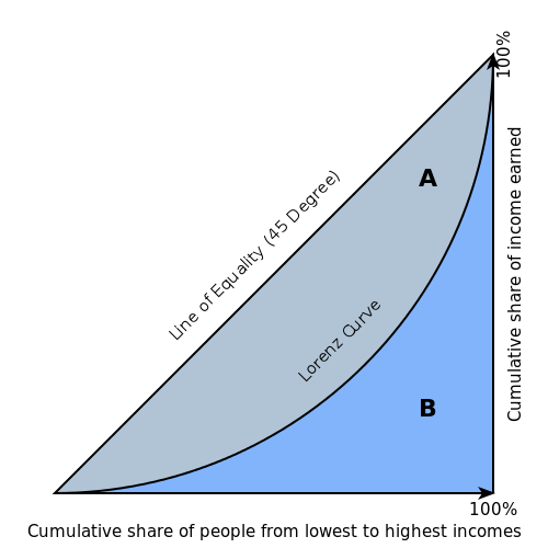
GINI (Gini Coefficient): The Gini index is a well-established method to quantify the inequality among values of a frequency distribution, and can be used to measure the quality of a binary classifier. A Gini index of zero expresses perfect equality (or a totally useless classifier), while a Gini index of one expresses maximal inequality (or a perfect classifier).

The Gini index is based on the Lorenz curve. The Lorenz curve plots the true positive rate (y-axis) as a function of percentiles of the population (x-axis).

The Lorenz curve represents a collective of models represented by the classifier. The location on the curve is given by the probability threshold of a particular model. (i.e., Lower probability thresholds for classification typically lead to more true positives, but also to more false positives.)

The Gini index itself is independent of the model and only depends on the Lorenz curve determined by the distribution of the scores (or probabilities) obtained from the classifier.

Regression¶

R2 (R Squared): The R2 value represents the degree that the predicted value and the actual value move in unison. The R2 value varies between 0 and 1 where 0 represents no correlation between the predicted and actual value and 1 represents complete correlation.

Calculating the R2 value for linear models is mathematically equivalent to \(1 - SSE/SST\) (or \(1 - \text{residual sum of squares}/\text{total sum of squares}\)). For all other models, this equivalence does not hold, so the \(1 - SSE/SST\) formula cannot be used. In some cases, this formula can produce negative R2 values, which is mathematically impossible for a real number. Because Driverless AI does not necessarily use linear models, the R2 value is calculated using the squared Pearson correlation coefficient.

R2 equation:

\[R2 = \frac{\sum_{i=1}^{n}(x_i-\bar{x})(y_i-\bar{y})}{\sqrt{\sum_{i=1}^{n}(x_i-\bar{x})^2\sum_{i=1}^{n}(y_i-\bar{y})^2}}\]

Where:

x is the predicted target value

y is the actual target value

MSE (Mean Squared Error): The MSE metric measures the average of the squares of the errors or deviations. MSE takes the distances from the points to the regression line (these distances are the “errors”) and squaring them to remove any negative signs. MSE incorporates both the variance and the bias of the predictor.

MSE also gives more weight to larger differences. The bigger the error, the more it is penalized. For example, if your correct answers are 2,3,4 and the algorithm guesses 1,4,3, then the absolute error on each one is exactly 1, so squared error is also 1, and the MSE is 1. But if the algorithm guesses 2,3,6, then the errors are 0,0,2, the squared errors are 0,0,4, and the MSE is a higher 1.333. The smaller the MSE, the better the model’s performance. (Tip: MSE is sensitive to outliers. If you want a more robust metric, try mean absolute error (MAE).)

MSE equation:

\[MSE = \frac{1}{N} \sum_{i=1}^{N}(y_i -\hat{y}_i)^2\]

RMSE (Root Mean Squared Error): The RMSE metric evaluates how well a model can predict a continuous value. The RMSE units are the same as the predicted target, which is useful for understanding if the size of the error is of concern or not. The smaller the RMSE, the better the model’s performance. (Tip: RMSE is sensitive to outliers. If you want a more robust metric, try mean absolute error (MAE).)

RMSE equation:

\[RMSE = \sqrt{\frac{1}{N} \sum_{i=1}^{N}(y_i -\hat{y}_i)^2 }\]

Where:

N is the total number of rows (observations) of your corresponding dataframe.

y is the actual target value.

\(\hat{y}\) is the predicted target value.

RMSLE (Root Mean Squared Logarithmic Error): This metric measures the ratio between actual values and predicted values and takes the log of the predictions and actual values. Use this instead of RMSE if an under-prediction is worse than an over-prediction. You can also use this when you don’t want to penalize large differences when both of the values are large numbers.

RMSLE equation:

\[RMSLE = \sqrt{\frac{1}{N} \sum_{i=1}^{N} \big(ln \big(\frac{y_i +1} {\hat{y}_i +1}\big)\big)^2 }\]

Where:

N is the total number of rows (observations) of your corresponding dataframe.

y is the actual target value.

\(\hat{y}\) is the predicted target value.

RMSPE (Root Mean Square Percentage Error): This metric is the RMSE expressed as a percentage. The smaller the RMSPE, the better the model performance.

RMSPE equation:

\[RMSPE = \sqrt{\frac{1}{N} \sum_{i=1}^{N} \frac{(y_i -\hat{y}_i)^2 }{(y_i)^2}}\]

MAE (Mean Absolute Error): The mean absolute error is an average of the absolute errors. The MAE units are the same as the predicted target, which is useful for understanding whether the size of the error is of concern or not. The smaller the MAE the better the model’s performance. (Tip: MAE is robust to outliers. If you want a metric that is sensitive to outliers, try root mean squared error (RMSE).)

MAE equation:

\[MAE = \frac{1}{N} \sum_{i=1}^{N} | x_i - x |\]

Where:
- N is the total number of errors
- \(| x_i - x |\) equals the absolute errors.

MAPE (Mean Absolute Percentage Error): MAPE measures the size of the error in percentage terms. It is calculated as the average of the unsigned percentage error.

MAPE equation:

\[MAPE = \big(\frac{1}{N} \sum \frac {|Actual - Forecast |}{|Actual|} \big) * 100\]

Because the MAPE measure is in percentage terms, it gives an indication of how large the error is across different scales. Consider the following example:

Actual Predicted Absolute Error Absolute Percentage Error

5 1 4 80%

15,000 15,004 4 0.03%

Both records have an absolute error of 4, but this error could be considered “small” or “big” when you compare it to the actual value.

SMAPE (Symmetric Mean Absolute Percentage Error): Unlike the MAPE, which divides the absolute errors by the absolute actual values, the SMAPE divides by the mean of the absolute actual and the absolute predicted values. This is important when the actual values can be 0 or near 0. Actual values near 0 cause the MAPE value to become infinitely high. Because SMAPE includes both the actual and the predicted values, the SMAPE value can never be greater than 200%.

Consider the following example:

Actual Predicted

0.01 0.05

0.03 0.04

The MAPE for this data is 216.67% but the SMAPE is only 80.95%.

Both records have an absolute error of 4, but this error could be considered “small” or “big” when you compare it to the actual value.

MER (Median Error Rate or Median Absolute Percentage Error): MER measures the median size of the error in percentage terms. It is calculated as the median of the unsigned percentage error.

MER equation:

\[MER = \big(median \frac {|Actual - Forecast |}{|Actual|} \big) * 100\]

Because the MER is the median, half the scored population has a lower absolute percentage error than the MER, and half the population has a larger absolute percentage error than the MER.

Classification¶

MCC (Matthews Correlation Coefficient): The goal of the MCC metric is to represent the confusion matrix of a model as a single number. The MCC metric combines the true positives, false positives, true negatives, and false negatives using the equation described below.

A Driverless AI model will return probabilities, not predicted classes. To convert probabilities to predicted classes, a threshold needs to be defined. Driverless AI iterates over possible thresholds to calculate a confusion matrix for each threshold. It does this to find the maximum MCC value. Driverless AI’s goal is to continue increasing this maximum MCC.

Unlike metrics like Accuracy, MCC is a good scorer to use when the target variable is imbalanced. In the case of imbalanced data, high Accuracy can be found by simply predicting the majority class. Metrics like Accuracy and F1 can be misleading, especially in the case of imbalanced data, because they do not consider the relative size of the four confusion matrix categories. MCC, on the other hand, takes the proportion of each class into account. The MCC value ranges from -1 to 1 where -1 indicates a classifier that predicts the opposite class from the actual value, 0 means the classifier does no better than random guessing, and 1 indicates a perfect classifier.

MCC equation:

\[MCC = \frac{TP \; x \; TN \; - FP \; x \; FN}{\sqrt{(TP+FP)(TP+FN)(TN+FP)(TN+FN)}}\]

F05, F1, and F2: A Driverless AI model will return probabilities, not predicted classes. To convert probabilities to predicted classes, a threshold needs to be defined. Driverless AI iterates over possible thresholds to calculate a confusion matrix for each threshold. It does this to find the maximum some F metric value. Driverless AI’s goal is to continue increasing this maximum F metric.

The F1 score provides a measure for how well a binary classifier can classify positive cases (given a threshold value). The F1 score is calculated from the harmonic mean of the precision and recall. An F1 score of 1 means both precision and recall are perfect and the model correctly identified all the positive cases and didn’t mark a negative case as a positive case. If either precision or recall are very low it will be reflected with a F1 score closer to 0.

F1 equation:

\[F1 = 2 \;\Big(\; \frac{(precision) \; (recall)}{precision + recall}\; \Big)\]

Where:

precision is the positive observations (true positives) the model correctly identified from all the observations it labeled as positive (the true positives + the false positives).

recall is the positive observations (true positives) the model correctly identified from all the actual positive cases (the true positives + the false negatives).

The F0.5 score is the weighted harmonic mean of the precision and recall (given a threshold value). Unlike the F1 score, which gives equal weight to precision and recall, the F0.5 score gives more weight to precision than to recall. More weight should be given to precision for cases where False Positives are considered worse than False Negatives. For example, if your use case is to predict which products you will run out of, you may consider False Positives worse than False Negatives. In this case, you want your predictions to be very precise and only capture the products that will definitely run out. If you predict a product will need to be restocked when it actually doesn’t, you incur cost by having purchased more inventory than you actually need.

F05 equation:

\[F0.5 = 1.25 \;\Big(\; \frac{(precision) \; (recall)}{0.25 \; precision + recall}\; \Big)\]

Where:

precision is the positive observations (true positives) the model correctly identified from all the observations it labeled as positive (the true positives + the false positives).

recall is the positive observations (true positives) the model correctly identified from all the actual positive cases (the true positives + the false negatives).

The F2 score is the weighted harmonic mean of the precision and recall (given a threshold value). Unlike the F1 score, which gives equal weight to precision and recall, the F2 score gives more weight to recall than to precision. More weight should be given to recall for cases where False Negatives are considered worse than False Positives. For example, if your use case is to predict which customers will churn, you may consider False Negatives worse than False Positives. In this case, you want your predictions to capture all of the customers that will churn. Some of these customers may not be at risk for churning, but the extra attention they receive is not harmful. More importantly, no customers actually at risk of churning have been missed.

F2 equation:

\[F2 = 5 \;\Big(\; \frac{(precision) \; (recall)}{4\;precision + recall}\; \Big)\]

Where:

precision is the positive observations (true positives) the model correctly identified from all the observations it labeled as positive (the true positives + the false positives).

recall is the positive observations (true positives) the model correctly identified from all the actual positive cases (the true positives + the false negatives).

Accuracy: In binary classification, Accuracy is the number of correct predictions made as a ratio of all predictions made. In multiclass classification, the set of labels predicted for a sample must exactly match the corresponding set of labels in y_true.

A Driverless AI model will return probabilities, not predicted classes. To convert probabilities to predicted classes, a threshold needs to be defined. Driverless AI iterates over possible thresholds to calculate a confusion matrix for each threshold. It does this to find the maximum Accuracy value. Driverless AI’s goal is to continue increasing this maximum Accuracy.

Accuracy equation:

\[Accuracy = \Big(\; \frac{\text{number correctly predicted}}{\text{number of observations}}\; \Big)\]

Logloss: The logarithmic loss metric can be used to evaluate the performance of a binomial or multinomial classifier. Unlike AUC which looks at how well a model can classify a binary target, logloss evaluates how close a model’s predicted values (uncalibrated probability estimates) are to the actual target value. For example, does a model tend to assign a high predicted value like .80 for the positive class, or does it show a poor ability to recognize the positive class and assign a lower predicted value like .50? Logloss ranges between 0 and 1, with 0 meaning that the model correctly assigns a probability of 0% or 100%.

Binary classification equation:

\[Logloss = - \;\frac{1}{N} \sum_{i=1}^{N}w_i(\;y_i \ln(p_i)+(1-y_i)\ln(1-p_i)\;)\]

Multiclass classification equation:

\[Logloss = - \;\frac{1}{N} \sum_{i=1}^{N}\sum_{j=1}^{C}w_i(\;y_i,_j \; \ln(p_i,_j)\;)\]

Where:

N is the total number of rows (observations) of your corresponding dataframe.

w is the per row user-defined weight (defaults is 1).

C is the total number of classes (C=2 for binary classification).

p is the predicted value (uncalibrated probability) assigned to a given row (observation).

y is the actual target value.

AUC (Area Under the Receiver Operating Characteristic Curve): This model metric is used to evaluate how well a binary classification model is able to distinguish between true positives and false positives. For multi-class problems, this score is computed by micro-averaging the ROC curves for each class. Use MACROAUC if you prefer the macro average.

An AUC of 1 indicates a perfect classifier, while an AUC of .5 indicates a poor classifier whose performance is no better than random guessing.

AUCPR (Area Under the Precision-Recall Curve): This model metric is used to evaluate how well a binary classification model is able to distinguish between precision recall pairs or points. These values are obtained using different thresholds on a probabilistic or other continuous-output classifier. AUCPR is an average of the precision-recall weighted by the probability of a given threshold.

The main difference between AUC and AUCPR is that AUC calculates the area under the ROC curve and AUCPR calculates the area under the Precision Recall curve. The Precision Recall curve does not care about True Negatives. For imbalanced data, a large quantity of True Negatives usually overshadows the effects of changes in other metrics like False Positives. The AUCPR will be much more sensitive to True Positives, False Positives, and False Negatives than AUC. As such, AUCPR is recommended over AUC for highly imbalanced data.

MACROAUC (Macro Average of Areas Under the Receiver Operating Characteristic Curves): For multiclass classification problems, this score is computed by macro-averaging the ROC curves for each class (one per class). The area under the curve is a constant. A MACROAUC of 1 indicates a perfect classifier, while a MACROAUC of .5 indicates a poor classifier whose performance is no better than random guessing. This option is not available for binary classification problems.

Scorer Best Practices - Regression¶

When deciding which scorer to use in a regression problem, some main questions to ask are:

Do you want your scorer sensitive to outliers?
What unit should the scorer be in?

Sensitive to Outliers

Certain scorers are more sensitive to outliers. When a scorer is sensitive to outliers, it means that it is important that the model predictions are never “very” wrong. For example, let’s say we have an experiment predicting number of days until an event. The graph below shows the absolute error in our predictions.

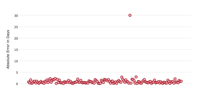
Usually our model is very good. We have an absolute error less than 1 day about 70% of the time. There is one instance, however, where our model did very poorly. We have one prediction that was 30 days off.

Instances like this will more heavily penalize scorers that are sensitive to outliers. If we do not care about these outliers in poor performance as long as we typically have a very accurate prediction, then we would want to select a scorer that is robust to outliers. We can see this reflected in the behavior of the scorers: MSE and RMSE.

	MSE	RMSE
Outlier	0.99	2.64
No Outlier	0.80	1.0

Calculating the RMSE and MSE on our error data, the RMSE is more than twice as large as the MSE because RMSE is sensitive to outliers. If we remove the one outlier record from our calculation, RMSE drops down significantly.

Performance Units

Different scorers will show the performance of the Driverless AI experiment in different units. Let’s continue with our example where our target is to predict the number of days until an event. Some possible performance units are:

Same as target: The unit of the scorer is in days
- ex: MAE = 5 means the model predictions are off by 5 days on average
Percent of target: The unit of the scorer is the percent of days
- ex: MAPE = 10% means the model predictions are off by 10 percent on average
Square of target: The unit of the scorer is in days squared
- ex: MSE = 25 means the model predictions are off by 5 days on average (square root of 25 = 5)

Comparison

Metric	Units	Sensitive to Outliers	Tip
R2	scaled between 0 and 1	No	use when you want perfor mance scaled betwee n 0 and 1
MSE	square of target	Yes
RMSE	same as target	Yes
RMSLE	log of target	Yes
RMSPE	percent of target	Yes	use when target values are across differ ent scales
MAE	same as target	No
MAPE	percent of target	No	use when target values are across differ ent scales
SMAPE	percent of target divided by 2	No	use when target values close to 0

Scorer Best Practices - Classification¶

When deciding which scorer to use in a classification problem some main questions to ask are:

Do you want the scorer to evaluate the predicted probabilities or the classes that those probabilities can be converted to?
Is your data imbalanced?

Scorer Evaluates Probabilities or Classes

The final output of a Driverless AI model is a predicted probability that a record is in a particular class. The scorer you choose will either evaluate how accurate the probability is or how accurate the assigned class is from that probability.

Choosing this depends on the use of the Driverless AI model. Do we want to use the probabilities or do we want to convert those probabilities into classes? For example, if we are predicting whether a customer will churn, we may take the predicted probabilities and turn them into classes - customers who will churn vs customers who won’t churn. If we are predicting the expected loss of revenue, we will instead use the predicted probabilities (predicted probability of churn * value of customer).

If your use case requires a class assigned to each record, you will want to select a scorer that evaluates the model’s performance based on how well it classifies the records. If your use case will use the probabilities, you will want to select a scorer that evaluates the model’s performance based on the predicted probability.

Robust to Imbalanced Data

For certain use cases, positive classes may be very rare. In these instances, some scorers can be misleading. For example, if I have a use case where 99% of the records have Class = No, then a model which always predicts No will have 99% accuracy.

For these use cases, it is best to select a metric that does not include True Negatives or considers relative size of the True Negatives like AUCPR or MCC.

Comparison

Metric	Evaluation Based On	Tip
MCC	Class	good for imbalanced data
F1	Class
F0.5	Class	good when you want to give more weight to precision
F2	Class	good when you want to give more weight to recall
Accuracy	Class	highly interpretable
Logloss	Probability
AUC	Class
AUCPR	Class	good for imbalanced data

New Experiments¶

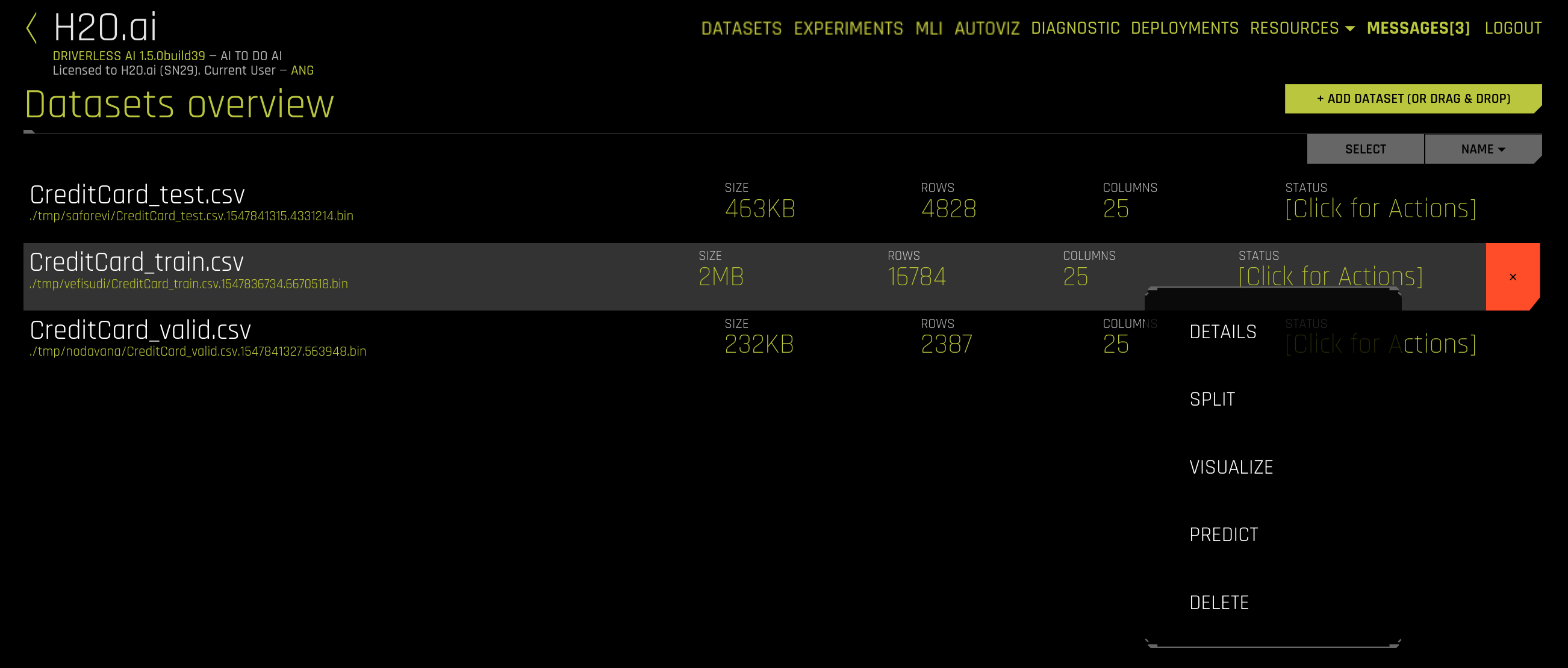
Run an experiment by selecting [Click for Actions] button beside the dataset that you want to use. Click Predict to begin an experiment.

The Experiment Settings form displays and auto-fills with the selected dataset. Optionally specify a validation dataset and/or a test dataset.

The validation set is used to tune parameters (models, features, etc.). If a validation dataset is not provided, the training data is used (with holdout splits). If a validation dataset is provided, training data is not used for parameter tuning - only for training. A validation dataset can help to improve the generalization performance on shifting data distributions.

The test dataset is used for the final stage scoring and is the dataset for which model metrics will be computed against. Test set predictions will be available at the end of the experiment. This dataset is not used during training of the modeling pipeline.

Keep in mind that these datasets must have the same number of columns as the training dataset. Also note that if provided, the validation set is not sampled down, so it can lead to large memory usage, even if accuracy=1 (which reduces the train size).

Specify the target (response) column. Note that not all explanatory functionality will be available for multiclass classification scenarios (scenarios with more than two outcomes). When the target column is selected, Driverless AI automatically provides the target column type and the number of rows. If this is a classification problem, then the UI shows unique and frequency statistics (Target Freq/Most Freq) for numerical columns. If this is a regression problem, then the UI shows the dataset mean and standard deviation values.

Notes Regarding Frequency:

For data imported in versions <= 1.0.19, TARGET FREQ and MOST FREQ both represent the count of the least frequent class for numeric target columns and the count of the most frequent class for categorical target columns.

For data imported in versions 1.0.20-1.0.22, TARGET FREQ and MOST FREQ both represent the frequency of the target class (second class in lexicographic order) for binomial target columns; the count of the most frequent class for categorical multinomial target columns; and the count of the least frequent class for numeric multinomial target columns.

For data imported in version 1.0.23 (and later), TARGET FREQ is the frequency of the target class for binomial target columns, and MOST FREQ is the most frequent class for multinomial target columns.

The next step is to set the parameters and settings for the experiment. (Refer to the Experiment Settings section for more information about these settings.) You can set the parameters individually, or you can let Driverless AI infer the parameters and then override any that you disagree with. Available parameters and settings include the following:

Dropped Columns: The columns we do not want to use as predictors such as ID columns, columns with data leakage, etc.

Weight Column: The column that indicates the per row observation weights. If “None” is specified, each row will have an observation weight of 1.

Fold Column: The column that indicates the fold. If “None” is specified, the folds will be determined by Driverless AI. This is set to “Disabled” if a validation set is used.

Time Column: The column that provides a time order, if applicable. If “AUTO” is specified, Driverless AI will auto-detect a potential time order. If “OFF” is specified, auto-detection is disabled. This is set to “Disabled” if a validation set is used.

Specify the scorer to use for this experiment. The scorers vary based on whether this is a classification or regression experiment. Available scorers include:

Regression: GINI, R2, MSE, RMSE (default), RMSLE, RMSPE, MAE, MER, MAPE, SMAPE

Classification: GINI, MCC, F05, F1, F2, ACCURACY, LOGLOSS, AUC (default), AUCPR

Desired relative Accuracy from 1 to 10

Desired relative Time from 1 to 10

Desired relative Interpretability from 1 to 10

Driverless AI will automatically infer the best settings for Accuracy, Time, and Interpretability and provide you with an experiment preview based on those suggestions. If you adjust these knobs, the experiment preview will automatically update based on the new settings.

Expert Settings (optional):

Optionally specify additional expert settings for the experiment. Refer to the Expert Settings section for more information about these settings. The default values for these options are derived from the environment variables in the config.toml file. Refer to the Setting Environment Variables section for more information.

Additional settings (optional):

Classification or Regression button. Driverless AI automatically determines the problem type based on the response column. Though not recommended, you can override this setting by clicking this button.

Reproducible: This button allows you to build an experiment with a random seed and get reproducible results. If this is disabled (default), then results will vary between runs.

Enable GPUs: Specify whether to enable GPUs. (Note that this option is ignored on CPU-only systems.)

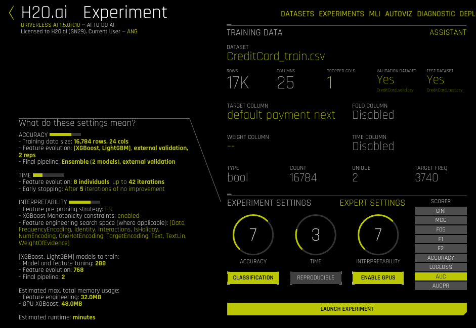
Click Launch Experiment to start the experiment.

The experiment launches with a randomly generated experiment name. You can change this name at anytime during or after the experiment. Mouse over the name of the experiment to view an edit icon, then type in the desired name.

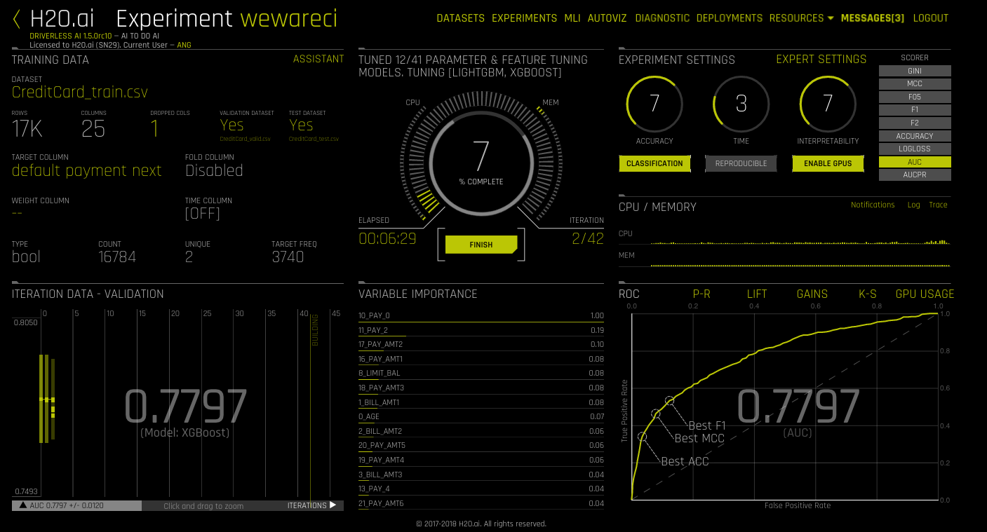
As the experiment runs, a running status displays in the upper middle portion of the UI. First Driverless AI figures out the backend and determines whether GPUs are running. Then it starts parameter tuning, followed by feature engineering. Finally, Driverless AI builds the scoring pipeline.

In addition to the status, the UI also displays:

Details about the dataset.

The iteration data (internal validation) for each cross validation fold along with the specified scorer value. Click on a specific iteration or drag to view a range of iterations. Double click in the graph to reset the view. In this graph, each “column” represents one iteration of the experiment. During the iteration, Driverless AI will train \(n\) models. (This is called individuals in the experiment preview.) So for any column, you may see the score value for those \(n\) models for each iteration on the graph.

The variable importance values. To view variable importance for a specific iteration, just select that iteration in the Iteration Data graph. The Variable Importance list will automatically update to show variable importance information for that iteration. Hover over an entry to view more info. Note: When hovering over an entry, you may notice the term “Internal[…] specification.” This label is used for features that do not need to be translated/explained and ensures that all features are uniquely identified.

CPU/Memory information including Notifications, Logs, and Trace info.

For classification problems, the lower right section includes a toggle between an ROC curve, Precision-Recall graph, Lift chart, Gains chart, and GPU Usage information (if GPUs are available). For regression problems, the lower right section includes a toggle between an Actual vs. Predicted chart and GPU Usage information (if GPUs are available). (Refer to the Experiment Graphs section for more information.) Upon completion, an Experiment Summary section will populate in the lower right section.

The bottom portion of the experiment screen will show any warnings that Driverless AI encounters. You can hide this pane by clicking the x icon.

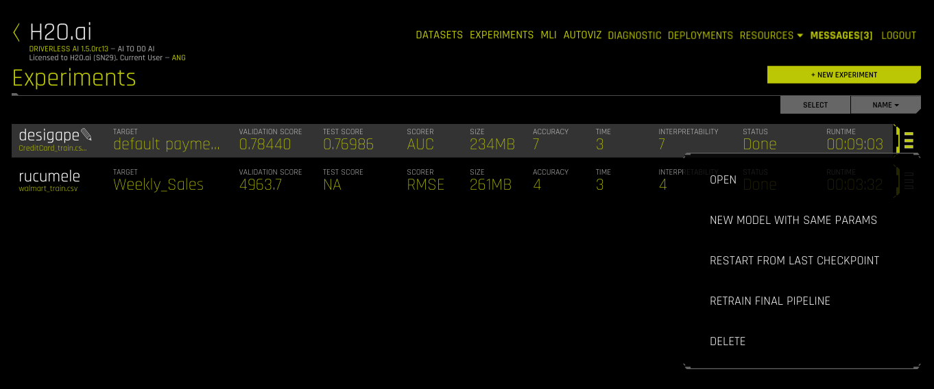
You can stop experiments that are currently running. Click the Finish button to stop the experiment. This jumps the experiment to the end and completes the ensembling and the deployment package. You can also click Abort to terminate the experiment. (You will be prompted to confirm the abort.) Aborted experiments will display on the Experiments page as Failed. You can restart aborted experiments by clicking the right side of the experiment, then selecting Restart from Last Checkpoint. This will start a new experiment based on the aborted one. Alternatively, you can started a new experiment based on the aborted one by selecting New Model with Same Params. Refer to Checkpointing, Rerunning, and Retraining for more information.

Experiment Graphs¶

This section describes the dashboard graphs that display for running and completed experiments. These graphs are interactive. Hover over a point on the graph for more details about the point.

Binary Classfication Experiments¶

For Binary Classification experiments, Driverless AI shows a ROC Curve, a Precision-Recall graph, a Lift chart, a Kolmogorov-Smirnov chart, and a Gains chart.

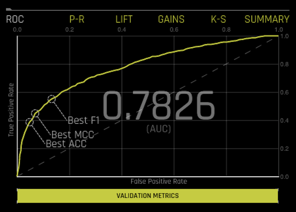
ROC: This shows Receiver-Operator Characteristics curve stats on validation data along with the best Accuracy, FCC, and F1 values.

The area under this curve is called AUC. The True Positive Rate (TPR) is the relative fraction of correct positive predictions, and the False Positive Rate (FPR) is the relative fraction of incorrect positive corrections. Each point corresponds to a classification threshold (e.g., YES if probability >= 0.3 else NO). For each threshold, there is a unique confusion matrix that represents the balance between TPR and FPR. Most useful operating points are in the top left corner in general.

Hover over a point in the ROC curve to see the True Positive, True Negative, False Positive, False Negative, Threshold, FPR, TPR, Accuracy, F1, and MCC value for that point.

If a test set was provided for the experiment, then click on the Validation Metrics button below the graph to view these stats on test data.

Precision-Recall: This shows the Precision-Recall curve on validation data along with the best Accuracy, FCC, and F1 values. The area under this curve is called AUCPR.

Precision: correct positive predictions (TP) / all positives (TP + FP).

Recall: correct positive predictions (TP) / positive predictions (TP + FN).

Each point corresponds to a classification threshold (e.g., YES if probability >= 0.3 else NO). For each threshold, there is a unique confusion matrix that represents the balance between Recall and Precision. This ROCPR curve can be more insightful than the ROC curve for highly imbalanced datasets.

Hover over a point in this graph to see the True Positive, True Negative, False Positive, False Negative, Threshold, Recall, Precision, Accuracy, F1, and MCC value for that point.

If a test set was provided for the experiment, then click on the Validation Metrics button below the graph to view these stats on test data.

Lift: This chart shows lift stats on validation data. For example, “How many times more observations of the positive target class are in the top predicted 1%, 2%, 10%, etc. (cumulative) compared to selecting observations randomly?” By definition, the Lift at 100% is 1.0.

Hover over a point in the Lift chart to view the quantile percentage and cumulative lift value for that point.

If a test set was provided for the experiment, then click on the Validation Metrics button below the graph to view these stats on test data.

Kolmogorov-Smirnov: This chart measures the degree of separation between positives and negatives for validation or test data.

Hover over a point in the chart to view the quantile percentage and Kolmogorov-Smirnov value for that point.

If a test set was provided for the experiment, then click on the Validation Metrics button below the graph to view these stats on test data.

Gains: This shows Gains stats on validation data. For example, “What fraction of all observations of the positive target class are in the top predicted 1%, 2%, 10%, etc. (cumulative)?” By definition, the Gains at 100% are 1.0.

Hover over a point in the Gains chart to view the quantile percentage and cumulative gain value for that point.

If a test set was provided for the experiment, then click on the Validation Metrics button below the graph to view these stats on test data.

Multiclass Classification Experiments¶

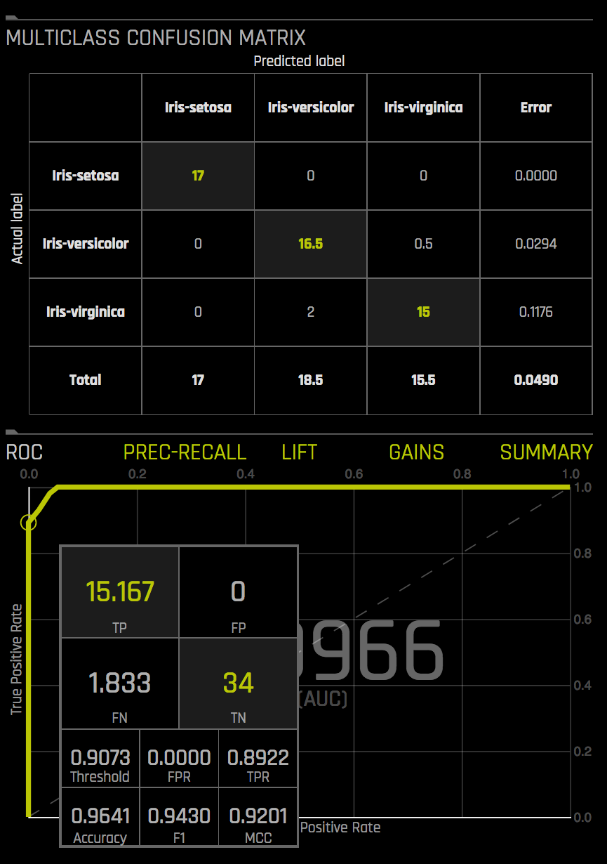
The ROC Curve, Precision-Recall graph, Lift chart, Kolmogorov-Smirnov chart, and Gains chart are also shown for multiclass problems. Driverless AI does this by considering the multi-class problem as multiple one-vs-all problems. This method is known as micro-averaging (reference: http://scikit-learn.org/stable/auto_examples/model_selection/plot_roc.html#multiclass-settings).

For example, you may want to predict the species in the iris data. The predictions would look something like this:

class.Iris-setosa	class.Iris-versicolor	class.Iris-virginica
0.9628	0.021	0.0158
0.0182	0.3172	0.6646
0.0191	0.9534	0.0276

To create these charts, Driverless AI converts the results to 3 one-vs-all problems:

prob-setosa	actual-setosa	prob-versicolor	actual-versicolor	prob-virginica	actual-virginica
0.9628	1	0.021	0	0.0158	0
0.0182	0	0.3172	1	0.6646	0
0.0191	0	0.9534	1	0.0276	0

The result is 3 vectors of predicted and actual values for binomial problems. Driverless AI concatenates these 3 vectors together to compute the charts.

predicted = [0.9628, 0.0182, 0.0191, 0.021, 0.3172, 0.9534, 0.0158, 0.6646, 0.0276]
actual = [1, 0, 0, 0, 1, 1, 0, 0, 0]

Multiclass Confusion Matrix¶

Hover over a point in the ROC or Precision Recall graph to view a Multiclass Confusion Matrix for that point (shown against the validation set). For each threshold, the confusion matrix represents the balance between TPR and FPR (ROC) or Precision and Recall (Prec-Recall). In general, most useful operating points are in the top left corner.

Regression Experiments¶

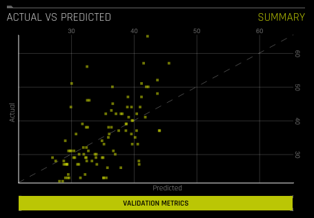
An Actual vs. Predicted table is available for Regression experiments. This shows Actual vs Predicted values on validation data. A small sample of values are displayed. A perfect model has a diagonal line.

Hover over a point on the graph to view the Actual and Predicted values for that point.

If a test set was provided for the experiment, then click on the Validation Metrics button below the graph to view these stats on test data.

Completed Experiment¶

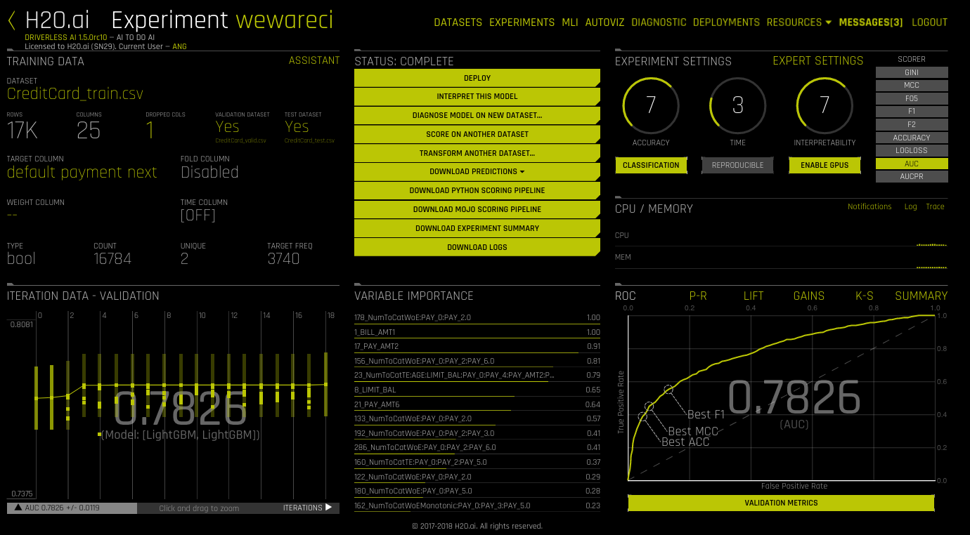
After an experiment status changes from RUNNING to COMPLETE, the UI provides you with several options:

Deploy: Refer to Deploying the MOJO Pipeline. (Only available after building MOJO scoring pipelines. Not available for PPC64LE environments.)

Interpret this Model: Refer to Interpreting a Model. (Not supported for NLP experiments. Please contact H2O support for assistance with interpreting NLP experiments.)

Diagnose Model on New Dataset: Refer to Diagnosing a Model.

Score on Another Dataset: Refer to Score on Another Dataset.

Transform Another Dataset: Refer to Transform Another Dataset. (Not available for Time Series experiments.)

Download Predictions dropdown:

Training (Holdout) Predictions: In csv format, available if a validation set was NOT provided. (Not available for Time Series experiments.)

Validation Set Predictions: In csv format, available if a validation set was provided.

Test Set Predictions: In csv format, available if a test dataset is used.

Download Python Scoring Pipeline: A standalone Python scoring pipeline for H2O Driverless AI. Refer to Driverless AI Standalone Python Scoring Pipeline.

Build MOJO Scoring Pipeline: A standalone Model Object, Optimized scoring pipeline. Refer to Driverless AI MOJO Scoring Pipeline. (Not available for TensorFlow, RuleFit, or FTRL models.)

Download Experiment Summary: A zip file containing the following files. Refer to the Experiment Summary section for more information.

A summary of the experiment

The experiment features along with their relative importance

Ensemble information

An experiment preview

Word version of an auto-generated report for the experiment

A target transformations tuning leaderboard

A tuning leaderboard

Download Logs

Experiment Summary¶

An experiment summary is available for each completed experiment. Click the Download Experiment Summary button to download the h2oai_experiment_summary_<experiment>.zip file.

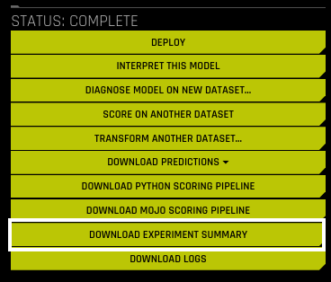
The files within the experiment summary zip provide textual explanations of the graphical representations that are shown on the Driverless AI UI. Details of each artifact are described below.

Experiment Report¶

A report file is included in the experiment summary. This report provides insight into the training data and any detected shifts in distribution, the validation schema selected, model parameter tuning, feature evolution and the final set of features chosen during the experiment.

report.docx: the report available in Word format

Click here to download and view a sample experiment report in Word format.

Experiment Overview Artifacts¶

The Experiment Summary contains artifacts that provide overviews of the experiment.

preview.txt: Provides a preview of the experiment. (This is the same information that was included on the UI before starting the experiment.)
summary.txt: Provides the same summary that appears in the lower-right portion of the UI for the experiment.
config.json: Provides a list of the settings used in the experiment.
args_do_auto_dl.json: The internal arguments used in the Driverless AI experiment based on the dataset and accuracy, time and interpretability settings.
experiment_column_types.json: Provides the column types for each column included in the experiment.
experiment_original_column.json: A list of all columns available in the dataset that was used in the experiment.
experiment_pipeline_original_required_columns.json: For columns used in the experiment, this incldes the column name and type.
experiment_sampling_description.json: A description of the sampling performed on the dataset.
timing.json: The timing and number of models generated in each part of the Driverless AI pipeline.
train_data_summary.csv: A summary of the training dataset used in the experiment.

Tuning Artifacts¶

During the Driverless AI experiment, model tuning is performed to determined the optimal algorithm and parameter settings for the provided dataset. For regression problems, target tuning is also performed to determine the best way to represent the target column (i.e. does taking the log of the target column improve results). The results from these tuning steps are available in the Experiment Summary.

tuning_leaderboard: A table of the model tuning performed along with the score generated from the model and training time. (Available in txt or json.)
target_transform_tuning_leaderboard.txt: A table of the transforms applied to the target column along with the score generated from the model and training time. (This will be empty for binary and multiclass use cases.)

Features Artifacts¶

Driverless AI performs feature engineering on the dataset to determine the optimal representation of the data. The top features used in the final model can be seen in the GUI. The complete list of features used in the final model is available in the Experiment Summary artifacts.

The Experiment Summary also provides a list of the original features and their estimated feature importance. For example, given the features in the final Driverless AI model, we can estimate the feature importance of the original features.

Feature Feature Importance

NumToCatWoE:PAY_AMT2 1

PAY_3 0.92

ClusterDist9:BILL_AMT1:LIMIT_BAL:PAY_3 0.90

To calculate the feature importance of PAY_3, we can aggregate the feature importance for all variables that used PAY_3:

NumToCatWoE:PAY_AMT2: 1 * 0 (PAY_3 not used.)
PAY_3: 0.92 * 1 (PAY_3 is the only variable used.)
ClusterDist9:BILL_AMT1:LIMIT_BAL:PAY_3: 0.90 * 1/3 (PAY_3 is one of three variables used.)

Estimated Feature Importance = (1*0) + (0.92*1) + (0.9*(1/3)) = 1.22

Note: The feature importance is converted to relative feature importance. (The feature with the highest estimated feature importance will have a relative feature importance of 1).

ensemble_features: A complete list of all features used in the final model, a description of the feature, and the relative feature importance. (Available in txt, table, or json.)
features_orig: A list of the original features provided and an estimate of the relative feature importance of that original feature in the final model. (Available in txt or json.)

Final Model Artifacts¶

The Experiment Summary includes artifacts that describe the final model. This is the model that is used to score new datasets and create the MOJO scoring pipeline. The final model may be an ensemble of models depending on the Accuracy setting.

ensemble.txt: A summary of the final model which includes a description of the model(s), gains/lifts table, confusion matrix, and scores of the final model for our list of scorers.
ensemble_description.txt: A sentence describing the final model. (For example: “Final TensorFlowModel pipeline with ensemble_level=0 transforming 21 original features -> 54 features in each of 1 models each fit on full training data (i.e. no hold-out).”)
ensemble_model_description.json: A json file describing the model(s) and for ensembles how the model predictions are weighted.
ensemble_model_params.json: A json file decribing the parameters of the model(s).
ensemble_folds_data.json: A json file describing the folds used for the final model(s). This includes the size of each fold of data and the performance of the final model on each fold. (Available if a fold column was specified.)
ensemble_features_orig: A list of the original features provided and an estimate of the relative feature importance of that original feature in the ensemble of models. (Available in txt or json.)
ensemble_features: A complete list of all features used in the final ensemble of models, a description of the feature, and the relative feature importance. (Available in txt, table, or json.)

The Experiment Summary also includes artifacts about the final model performance.

ensemble_scores.json: The scores of the final model for our list of scorers.
ensemble_confusion_matrix: The confusion matrix for the internal validation and test data if test data is provided.
ensemble_confusion_matrix_stats_test.json: Confusion matrix statistics on the test data. (Only available if test data provided)
ensemble_gains: The lift and gains table for the internal validation and test data if test data is provided. (Visualization of lift and gains can be seen in the UI.)
ensemble_roc: The ROC and Precision Recall table for the internal validation and test data if test data is provided. (Visualization of ROC and Precision Recall curve can be seen in the UI.)

Viewing Experiments¶

The upper-right corner of the Driverless AI UI includes an Experiments link.

Click this link to open the Experiments page. From this page, you can rename an experiment, view previous experiments, begin a new experiment, rerun an experiment, and delete an experiment.

Checkpointing, Rerunning, and Retraining¶

In Driverless AI, you can retry an experiment from the last checkpoint, you can run a new experiment using an existing experiment’s settings, and you can retrain an experiment’s final pipeline.

Checkpointing Experiments¶

In real-world scenarios, data can change. For example, you may have a model currently in production that was built using 1 million records. At a later date, you may receive several hundred thousand more records. Rather than building a new model from scratch, Driverless AI includes H2O.ai Brain, which enables caching and smart re-use of prior models to generate features for new models.

You can configure one of the following Brain levels in the experiment’s Expert Settings.

-1: Don’t use any brain cache
0: Don’t use any brain cache but still write to cache
1: Smart checkpoint if an old experiment_id is passed in (for example, via running “resume one like this” in the GUI)
2: Smart checkpoint if the experiment matches all column names, column types, classes, class labels, and time series options identically. (default)
3: Smart checkpoint like level #1, but for the entire population. Tune only if the brain population is of insufficient size.
4: Smart checkpoint like level #2, but for the entire population. Tune only if the brain population is of insufficient size.
5: Smart checkpoint like level #4, but will scan over the entire brain cache of populations (starting from resumed experiment if chosen) in order to get the best scored individuals.

If you chooses Level 2 (default), then Level 1 is also done when appropriate.

To make use of smart checkpointing, be sure that the new data has:

The same data column names as the old experiment
The same data types for each column as the old experiment. (This won’t match if, e.g,. a column was all int and then had one string row.)
The same target as the old experiment
The same target classes (if classification) as the old experiment
For time series, all choices for intervals and gaps must be the same

When the above conditions are met, then you can:

Start the same kind of experiment, just rerun for longer.
Use a smaller or larger data set (i.e. fewer or more rows).
Effectively do a final ensemble re-fit by varying the data rows and starting an experiment with a new accuracy, time=1, and interpretability. Check the experiment preview for what the ensemble will be.
Restart/Resume a cancelled, aborted, or completed experiment

To run smart checkpointing on an existing experiment, click the right side of the experiment that you want to retry, then select Restart from Last Checkpoint. The experiment settings page opens. Specify the new dataset. If desired, you can also change experiment settings, though the target column must be the same. Click Launch Experiment to resume the experiment from the last checkpoint and build a new experiment.

The smart checkpointing continues by adding a prior model as another model used during tuning. If that prior model is better (which is likely if it was run for more iterations), then that smart checkpoint model will be used during feature evolution iterations and final ensemble.

Notes:

Driverless AI does not guarantee exact continuation, only smart continuation from any last point.
The directory where the H2O.ai Brain meta model files are stored is tmp/H2O.ai_brain. In addition, the default maximum brain size is 20GB. Both the directory and the maximum size can be changed in the config.toml file.

Rerunning Experiments¶

To run a new experiment using an existing experiment’s settings, click the right side of the experiment that you want to use as the basis for the new experiment, then select New Model with Same Params. This opens the experiment settings page. From this page, you can rerun the experiment using the original settings, or you can specify to use new data and/or specify different experiment settings. Click Launch Experiment to create a new experiment with the same options.

Retrain Final Pipeline¶

To retrain an experiment’s final pipeline, click the right side of the experiment that you want to use as the basis for the new experiment, then select Retrain Final Pipeline. This opens the experiment settings page with the same settings as the original experiment except that Time is set to 0.

Deleting Experiments¶

To delete an experiment, click the right side of the experiment that you want to remove, then select Delete. A confirmation message will display asking you to confirm the delete. Click OK to delete the experiment or Cancel to return to the experiments page without deleting.