MLI for Time-Series Experiments

This section describes how to run MLI for time-series experiments. Refer to MLI for Regular (Non-Time-Series) Experiments for MLI information with regular experiments.

There are two methods you can use for interpreting time-series models:

• Using the Interpret this Model button on a completed experiment page to interpret a Driverless AI model on original and transformed features. (See below.)

• Using the MLI link in the upper right corner of the UI to interpret either a Driverless AI model or an external model. This process is described in the Model Interpretation on Driverless AI Models and Model Interpretation on External Models sections.

Limitations

• This release deprecates experiments run in 1.7.0 and earlier. MLI will not be available for experiments from versions <= 1.7.0.

• MLI is not available for NLP experiments or for multiclass Time Series.

• When the test set contains actuals, you will see the time series metric plot and the group metrics table. If there are no actuals, MLI will run, but you will see only the prediction value time series and a Shapley table.

• MLI does not require an Internet connection to run on current models.

Multi-Group Time Series MLI

This section describes how to run MLI on time series data for multiple groups.

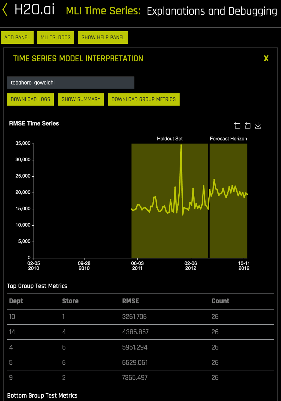
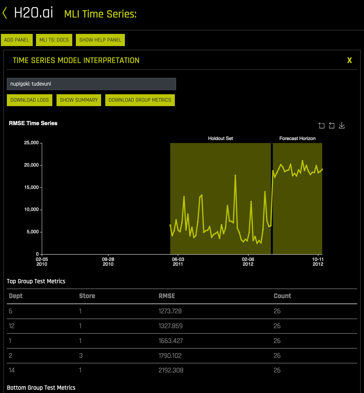
1. Click the Interpret this Model button on a completed time series experiment to launch Model Interpretation for that experiment. This page includes the following:

• A Help panel describing how to read and use this page. Click the Hide Help Button to hide this text.

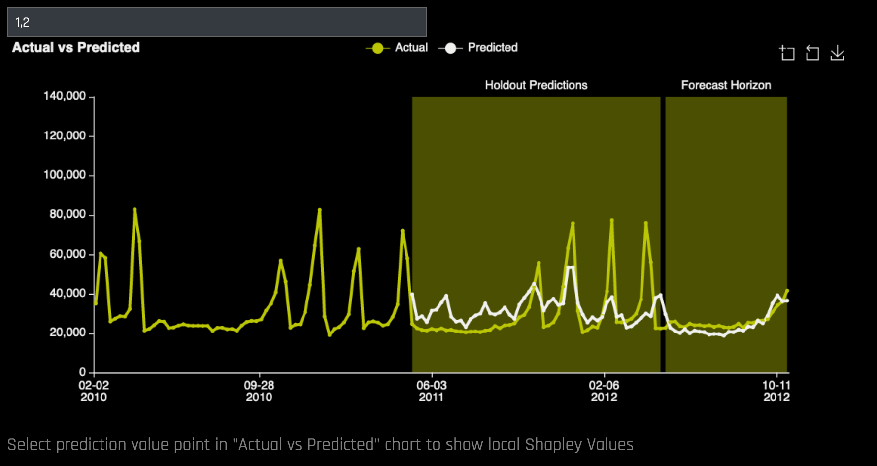
• If a test set is provided and the test set includes actuals, then a panel will display showing a time series plot and the top and bottom group matrix tables based on the scorer that was used in the experiment. The metric plot will show the metric of interest per time point for holdout predictions and the test set. Likewise, the actual vs. predicted plot will show actuals vs. predicted values per time point for the holdout set and the test set. Note that this panel can be resized if necessary.

• If a test set is not provided, then internal validation predictions will be used. The metric plot will only show the metric of interest per time point for holdout predictions. Likewise, the actual vs. predicted plot will only show actuals vs. predicted values per time point for the holdout set.

• A Download Logs button for retrieving logs that were generated when this interpretation was built.

• A Download Group Metrics button for retrieving the averages of each group’s scorer, as well as each group’s sample size.

• A Show Summary button that provide details about the experiment settings that were used.

• A Group Search entry field (scroll to bottom) for selecting the groups to view.

• Use the zoom feature to magnify any portion of a graph by clicking the Enable Zoom icon near the top-right corner of a graph. While this icon is selected, click and drag to draw a box over the portion of the graph you want to magnify. Click the Disable Zoom icon to return to the default view.

2. Scroll to the bottom of the panel and select a grouping in the Group Search field to view a graph of Actual vs. Predicted values for the group. The outputted graph can be downloaded to your local machine.

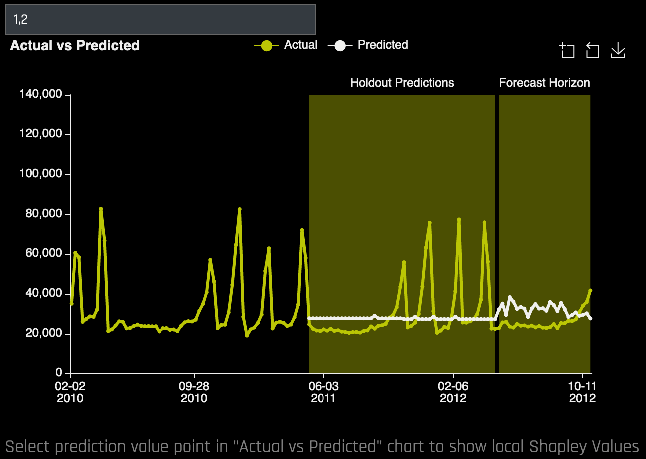
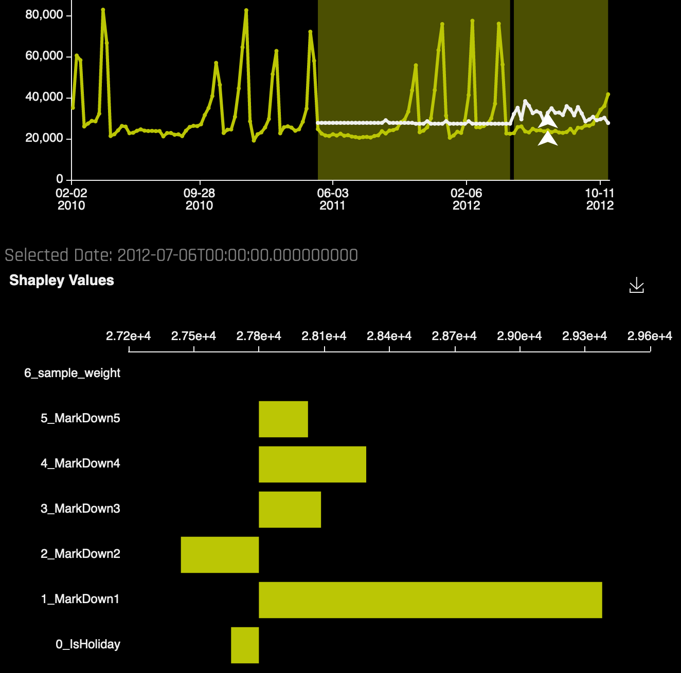
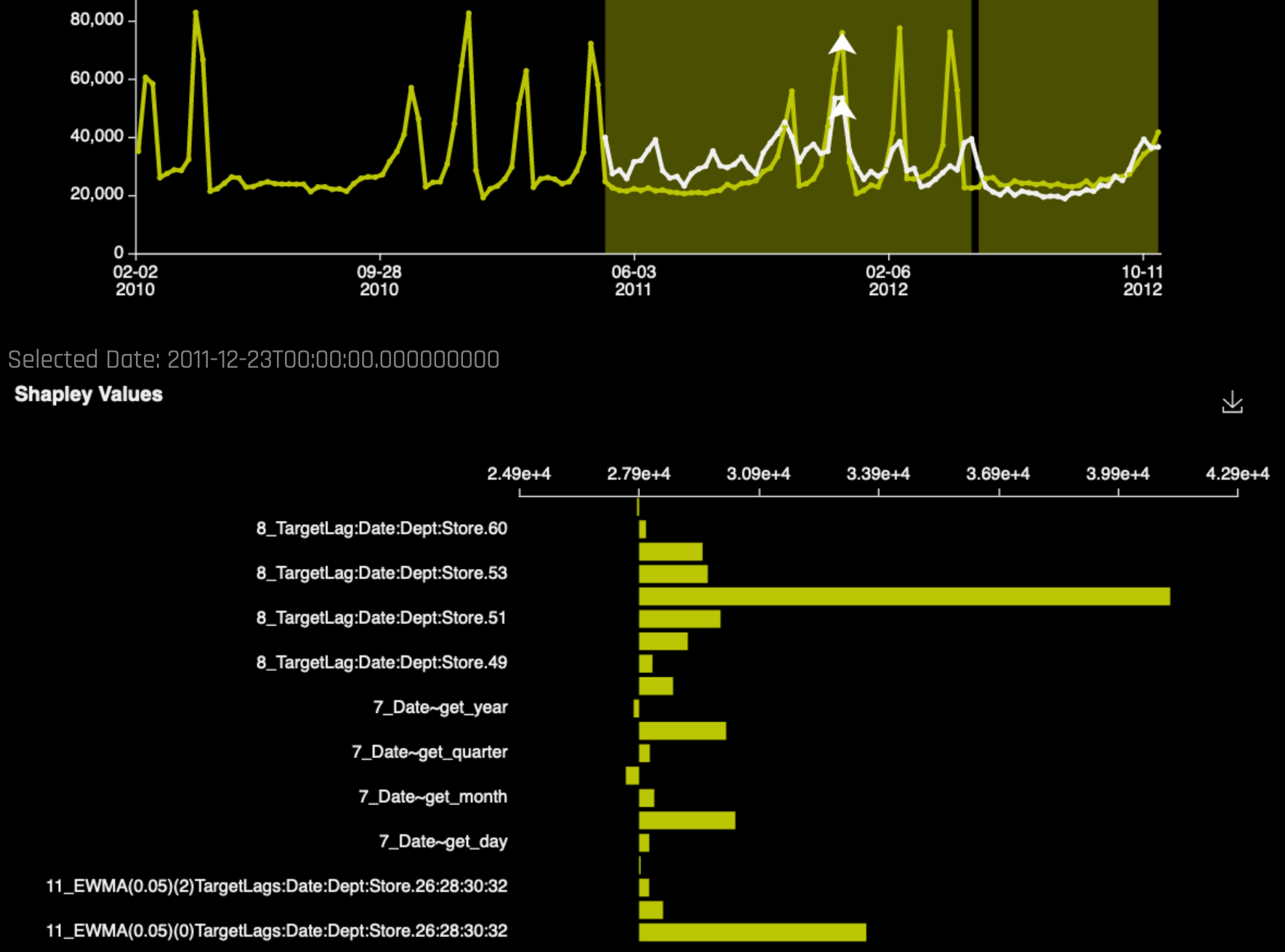
3. Click on a prediction point in the plot (white line) to view Shapley values for that prediction point. The Shapley values plot can also be downloaded to your local machine.

4. Click Add Panel to add a new MLI Time Series panel. This allows you to compare different groups in the same model and also provides the flexibility to do a “side-by-side” comparison between different models.

Single Time Series MLI

Time Series MLI can also be run when only one group is available.

1. Click the Interpret this Model button on a completed time series experiment to launch Model Interpretation for that experiment. This page includes the following:

• A Help panel describing how to read and use this page. Click the Hide Help Button to hide this text.

• If a test set is provided and the test set includes actuals, then a panel will display showing a time series plot and the top and bottom group matrix tables based on the scorer that was used in the experiment. The metric plot will show the metric of interest per time point for holdout predictions and the test set. Likewise, the actual vs. predicted plot will show actuals vs. predicted values per time point for the holdout set and the test set. Note that this panel can be resized if necessary.

• If a test set is not provided, then internal validation predictions will be used. The metric plot will only show the metric of interest per time point for holdout predictions. Likewise, the actual vs. predicted plot will only show actuals vs. predicted values per time point for the holdout set.

• A Download Logs button for retrieving logs that were generated when this interpretation was built.

• A Download Group Metrics button for retrieving the average of the group’s scorer, as well as the group’s sample size.

• A Show Summary button that provides details about the experiment settings that were used.

• A Group Search entry field for selecting the group to view. Note that for Single Time Series MLI, there will only be one option in this field.

• Use the zoom feature to magnify any portion of a graph by clicking the leftmost square icon near the top-right corner of a graph. While this icon is selected, click and drag to draw a box over the portion of the graph you want to magnify. To return to the default view, click the square-shaped arrow icon to the right of the zoom icon.

2. Scroll to the bottom of the panel and select an option in the Group Search field to view a graph of Actual vs. Predicted values for the group. (Note that for Single Time Series MLI, there will only be one option in this field.) The outputted graph can be downloaded to your local machine.

3. Click on a prediction point in the plot (white line) to view Shapley values for that prediction point. The Shapley values plot can also be downloaded to your local machine.

4. Click Add Panel to add a new MLI Time Series panel. This allows you to do a “side-by-side” comparison between different models.