Time Series in Driverless AI

Time series forecasting is one of the most common and important tasks in business analytics. There are many real-world applications like sales, weather, stock market, and energy demand, just to name a few. At H2O, we believe that automation can help our users deliver business value in a timely manner. Therefore, we combined advanced time series analysis and our Kaggle Grand Masters’ time series recipes into Driverless AI.

The key features/recipes that make automation possible are:

• Automatic handling of time groups (e.g., different stores and departments)

• Robust time series validation

  • Accounts for gaps and forecast horizon

  • Uses past information only (i.e., no data leakage)

• Time series-specific feature engineering recipes

  • Date features like day of week, day of month, etc.

  • AutoRegressive features, like optimal lag and lag-features interaction

  • Different types of exponentially weighted moving averages

  • Aggregation of past information (different time groups and time intervals)

  • Target transformations and differentiation

• Integration with existing feature engineering functions (recipes and optimization)

• Rolling-window based predictions for time series experiments with test-time augmentation or re-fit

• Automatic pipeline generation (See “From Kaggle Grand Masters’ Recipes to Production Ready in a Few Clicks” blog post.)

Note

Locale-dependent datetime formats may cause issues in Driverless AI. Converting datetime to a locale-independent format prior to running experiments is recommended. For information on how to convert datetime formats so that they are accepted in DAI, refer to the final note in the Modify by custom data recipe section.

Understanding Time Series

The following is an in depth description of time series in Driverless AI. For an overview of best practices when running time series experiments, see Time Series Best Practices.

Modeling Approach

Driverless AI uses GBMs, GLMs and neural networks with a focus on time series-specific feature engineering. The feature engineering includes:

• Autoregressive elements: creating lag variables

• Aggregated features on lagged variables: moving averages, exponential smoothing descriptive statistics, correlations

• Date-specific features: week number, day of week, month, year

• Target transformations: Integration/Differentiation, univariate transforms (like logs, square roots)

This approach is combined with AutoDL features as part of the genetic algorithm. The selection is still based on validation accuracy. In other words, the same transformations/genes apply; plus there are new transformations that come from time series. Some transformations (like target encoding) are deactivated.

When running a time series experiment, Driverless AI builds multiple models by rolling the validation window back in time (and potentially using less and less training data).

User-Configurable Options

Gap

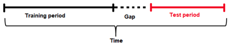
The guiding principle for properly modeling a time series forecasting problem is to use the historical data in the model training dataset such that it mimics the data/information environment at scoring time (i.e. deployed predictions). Specifically, you want to partition the training set to account for: 1) the information available to the model when making predictions and 2) the number of units out that the model should be optimized to predict.

Given a training dataset, the gap and forecast horizon are parameters that determine how to split the training dataset into training samples and validation samples.

Gap is the amount of missing time bins between the end of a training set and the start of test set (with regards to time). For example:

• Assume there are daily data with days 1/1/2020, 2/1/2020, 3/1/2020, 4/1/2020 in train. There are 4 days in total for training.

• In addition, the test data will start from 6/1/2020. There is only 1 day in the test data.

• The previous day (5/1/2020) does not belong to the train data. It is a day that cannot be used for training (i.e because information from that day may not be available at scoring time). This day cannot be used to derive information (such as historical lags) for the test data either.

• Here the time bin (or time unit) is 1 day. This is the time interval that separates the different samples/rows in the data.

• In summary, there are 4 time bins/units for the train data and 1 time bin/unit for the test data plus the Gap.

• In order to estimate the Gap between the end of the train data and the beginning of the test data, the following formula is applied.

• Gap = min(time bin test) - max(time bin train) - 1.

• In this case min(time bin test) is 6 (or 6/1/2020). This is the earliest (and only) day in the test data.

• max(time bin train) is 4 (or 4/1/2020). This is the latest (or the most recent) day in the train data.

• Therefore the GAP is 1 time bin (or 1 day in this case), because Gap = 6 - 4 - 1 or Gap = 1

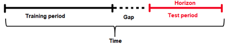
Forecast Horizon

It’s often not possible to have the most recent data available when applying a model (or it’s costly to update the data table too often); therefore some models need to be built accounting for a “future gap”. For example, if it takes a week to update a specific data table, you ideally want to predict 7 days ahead with the data as it is “today”; therefore a gap of 6 days is recommended. Not specifying a gap and predicting 7 days ahead with the data as it is is unrealistic (and cannot happen, as the data is updated on a weekly basis in this example). Similarly, gap can be used if you want to forecast further in advance. For example, if you want to know what will happen 7 days in the future, then set the gap to 6 days.

Forecast Horizon (or prediction length) is the period that the test data spans for (for example, one day, one week, etc.). In other words it is the future period that the model can make predictions for (or the number of units out that the model should be optimized to predict). Forecast horizon is used in feature selection and engineering and in model selection. Note that forecast horizon might not equal the number of predictions. The actual predictions are determined by the test dataset.

The periodicity of updating the data may require model predictions to account for significant time in the future. In an ideal world where data can be updated very quickly, predictions can always be made having the most recent data available. In this scenario there is no need for a model to be able to predict cases that are well into the future, but rather focus on maximizing its ability to predict short term. However this is not always the case, and a model needs to be able to make predictions that span deep into the future because it may be too costly to make predictions every single day after the data gets updated.

In addition, each future data point is not the same. For example, predicting tomorrow with today’s data is easier than predicting 2 days ahead with today’s data. Hence specifying the forecast horizon can facilitate building models that optimize prediction accuracy for these future time intervals.

Prediction Intervals

For regression problems, enable the prediction_intervals expert setting to have Driverless AI provide two additional columns y.lower and y.upper in the prediction frame. The true target value y for a predicted sample is expected to lie within [y.lower, y.upper] with a certain probability. The default value for this confidence level can be specified with the prediction_intervals_alpha expert setting, which has a default value of 0.9.

Driverless AI uses holdout predictions to determine intervals empirically (Williams, W.H. and Goodman, M.L. “A Simple Method for the Construction of Empirical Confidence Limits for Economic Forecasts.” Journal of the American Statistical Association, 66, 752-754. 1971). This method makes no assumption about the underlying model or the distribution of error and has been shown to outperform many other approaches (Lee, Yun Shin and Scholtes, Stefan. “Empirical prediction intervals revisited.” International Journal of Forecasting, 30, 217-234. 2014).

Notes:

• This feature applies to regression tasks (i.i.d. and time series).

• This feature works with all model types.

• Prediction intervals are computed for each individual time group.

time_period_in_seconds

Note: time_period_in_seconds is only available in the Python and R clients. Time period in seconds cannot be specified in the UI.

In Driverless AI, the forecast horizon (a.k.a., num_prediction_periods) needs to be in periods, and the size is unknown. To overcome this, you can use the optional time_period_in_seconds parameter when running start_experiment_sync (in Python) or train (in R). This is used to specify the forecast horizon in real time units (as well as for gap.) If this parameter is not specified, then Driverless AI will automatically detect the period size in the experiment, and the forecast horizon value will respect this period. I.e., if you are sure that your data has a 1 week period, you can say num_prediction_periods=14; otherwise it is possible that the model will not work correctly.

Groups

Groups are categorical columns in the data that can significantly help predict the target variable in time series problems. For example, one may need to predict sales given information about stores and products. Being able to identify that the combination of store and products can lead to very different sales is key for predicting the target variable, as a big store or a popular product will have higher sales than a small store and/or with unpopular products.

For example, if we don’t know that the store is available in the data, and we try to see the distribution of sales along time (with all stores mixed together), it may look like that:

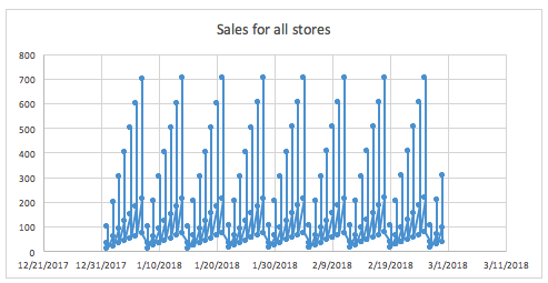
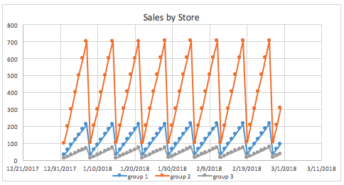
The same graph grouped by store gives a much clearer view of what the sales look like for different stores.

Lag

The primary generated time series features are lag features, which are a variable’s past values. At a given sample with time stamp \(t\), features at some time difference \(T\) (lag) in the past are considered. For example, if the sales today are 300, and sales of yesterday are 250, then the lag of one day for sales is 250. Lags can be created on any feature as well as on the target.

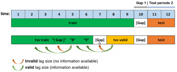
As previously noted, the training dataset is appropriately split such that the amount of validation data samples equals that of the testing dataset samples. If we want to determine valid lags, we must consider what happens when we will evaluate our model on the testing dataset. Essentially, the minimum lag size must be greater than the gap size.

Aside from the minimum useable lag, Driverless AI attempts to discover predictive lag sizes based on auto-correlation.

“Lagging” variables are important in time series because knowing what happened in different time periods in the past can greatly facilitate predictions for the future. Consider the following example to see the lag of 1 and 2 days:

Date	Sales	Lag1	Lag2
1/1/2020	100	-	-
2/1/2020	150	100	-
3/1/2020	160	150	100
4/1/2020	200	160	150
5/1/2020	210	200	160
6/1/2020	150	210	200
7/1/2020	160	150	210
8/1/2020	120	160	150
9/1/2020	80	120	160
10/1/2020	70	80	120

Time series target transformations

The following is a description of time series target transformations. These can be set through the Expert Settings window or by editing the config.toml file. For more information, see Using Driverless AI configuration options.

Note: Driverless AI does not attempt time series target transformations automatically; they must be set manually.

ts_lag_target_trafo (ts_lag_target_trafo): With this target transformation, you can select between the difference and ratio of the current and a lagged target. You can specify the corresponding lag size with the Lag size used for time series target transformation (ts_target_trafo_lag_size) setting.

Note: This target transformation can be used together with the Time series centering or detrending transformation (ts_target_trafo) target transformation, but it is mutually exclusive with regular target transformations.

ts_target_trafo (ts_target_trafo): With this target transformation, the free parameters of the trend model are fitted. The trend is removed from the target signal, and the pipeline is fitted on the residuals. Predictions are then made by adding back the trend.

Select one of the following options:

• none

• centering (fast)

• centering (robust)

• linear (fast)

• linear (robust)

• logistic

• epidemic

Notes:

• This target transformation can be used together with the Time series lag-based target transformation (ts_lag_target_trafo), but it is mutually exclusive with regular target transformations.

• The centering (robust) and linear (robust) detrending variants use scikit-learn’s implementation of random sample consensus (RANSAC) to achieve a higher tolerance with regard to outliers. As stated on scikit-learn’s page on robust linear model estimation using RANSAC, “The ordinary linear regressor is sensitive to outliers, and the fitted line can easily be skewed away from the true underlying relationship of data. The RANSAC regressor automatically splits the data into inliers and outliers, and the fitted line is determined only by the identified inliers.”

Settings Determined by Driverless AI

Window/Moving Average

Using the above Lag table, a moving average of 2 would constitute the average of Lag1 and Lag2:

Date	Sales	Lag1	Lag2	MA2
1/1/2020	100	-	-	-
2/1/2020	150	100	-	-
3/1/2020	160	150	100	125
4/1/2020	200	160	150	155
5/1/2020	210	200	160	180
6/1/2020	150	210	200	205
7/1/2020	160	150	210	180
8/1/2020	120	160	150	155
9/1/2020	80	120	160	140
10/1/2020	70	80	120	100

Aggregating multiple lags together (instead of just one) can facilitate stability for defining the target variable. It may include various lags values, for example lags [1-30] or lags [20-40] or lags [7-70 by 7].

Exponential Weighting

Exponential weighting is a form of weighted moving average where more recent values have higher weight than less recent values. That weight is exponentially decreased over time based on an alpha (a) (hyper) parameter (0,1), which is normally within the range of [0.9 - 0.99]. For example:

• Exponential Weight = a**(time)

• If sales 1 day ago = 3.0 and 2 days ago =4.5 and a=0.95:

• Exp. smooth = 3.0*(0.95**1) + 4.5*(0.95**2) / ((0.95**1) + (0.95**2)) =3.73 approx.

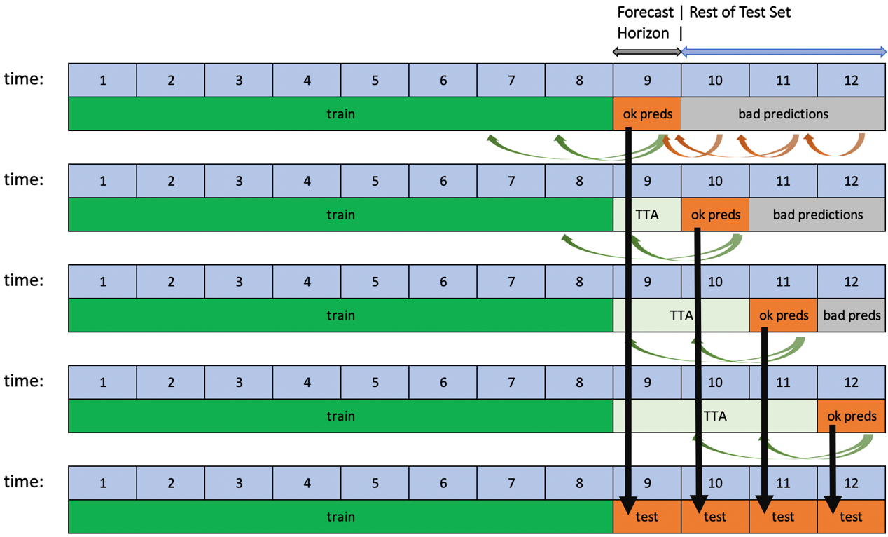
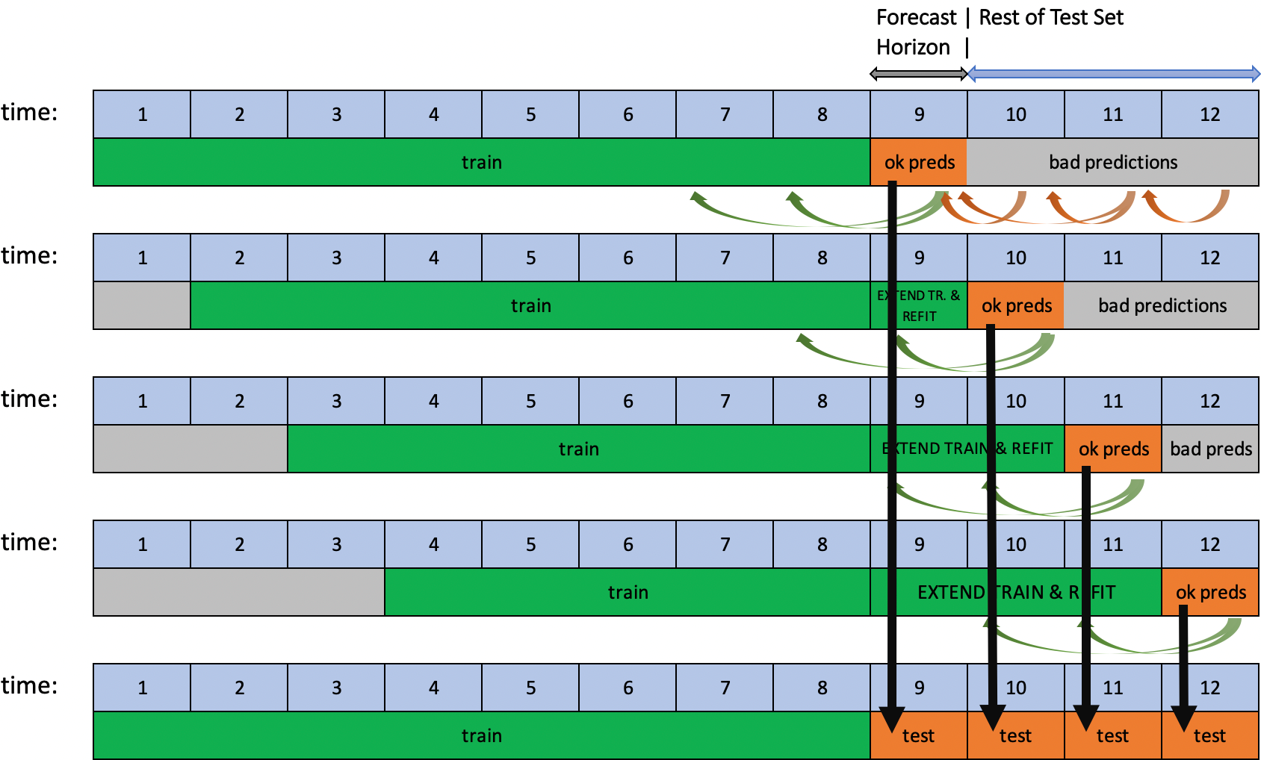
Rolling-Window-Based Predictions

Driverless AI supports rolling-window-based predictions for time series experiments with two options: Test Time Augmentation (TTA) or re-fit.

Both options are useful to assess the performance of the pipeline for predicting not just a single forecast horizon, but many in succession. TTA simulates the process where the model stays the same but the features are refreshed using newly available data. Re-fit simulates the process of re-fitting the entire pipeline (including the model) once new data is available.

This process is automated when the test set spans for a longer period than the forecast horizon and if the target values of the test set are known. If the user scores a test set that meets these conditions after the experiment is finished, rolling predictions with TTA will be applied. Re-fit, on the other hand, is only applicable for test sets provided during an experiment.

TTA is the default option and can be changed with the Method to Create Rolling Test Set Predictions expert setting.

Time Series Constraints

Dataset Size

Usually, the forecast horizon (prediction length) \(H\) equals the number of time periods in the testing data \(N_{TEST}\) (i.e. \(N_{TEST} = H\)). You want to have enough training data time periods \(N_{TRAIN}\) to score well on the testing dataset. At a minimum, the training dataset should contain at least three times as many time periods as the testing dataset (i.e. \(N_{TRAIN} >= 3 × N_{TEST}\)). This allows for the training dataset to be split into a validation set with the same amount of time periods as the testing dataset while maintaining enough historical data for feature engineering.

Time Series Use Case: Sales Forecasting

Below is a typical example of sales forecasting based on the Walmart competition on Kaggle. In order to frame it as a machine learning problem, we formulate the historical sales data and additional attributes as shown below:

Raw data

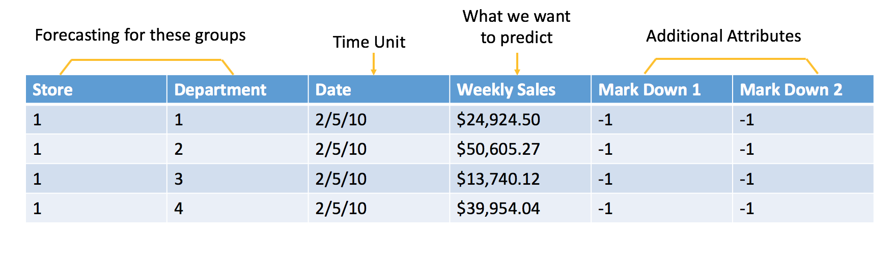
Data formulated for machine learning

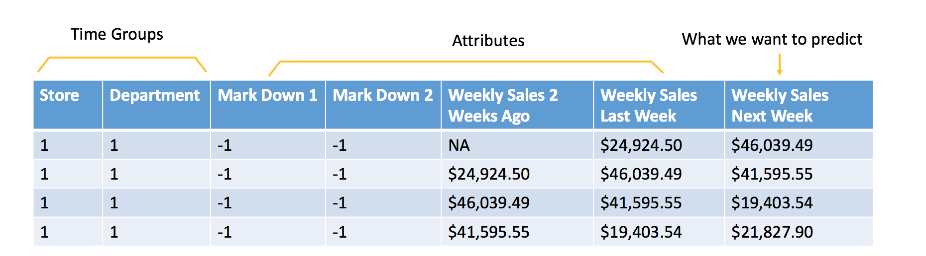
The additional attributes are attributes that we will know at time of scoring. In this example, the goal is to forecast the next week of sales, so all of the attributes included in the data must be known at least one week in advance. In this case, you can assume that you will know whether or not a Store and Department will be running a promotional markdown. Features like the temperature of the Week are not used because that information is not available at the time of scoring.

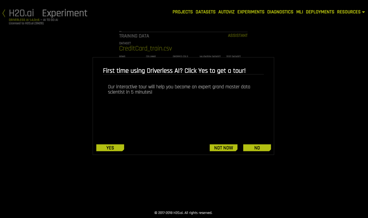
Once you have your data prepared in tabular format (see raw data above), Driverless AI can formulate it for machine learning and sort out the rest. If this is your very first session, the Driverless AI assistant will guide you through the journey.

Similar to previous Driverless AI examples, you need to select the dataset for training/test and define the target. For time series, you need to define the time column (by choosing AUTO or selecting the date column manually). If weighted scoring is required (like the Walmart Kaggle competition), you can select the column with specific weights for different samples.

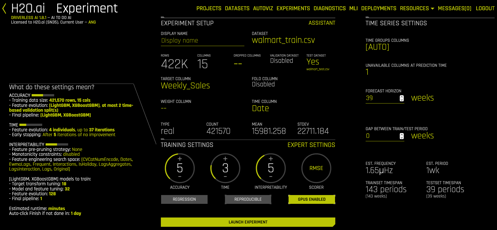
If you prefer to use automatic handling of time groups, you can leave the setting for time groups columns as AUTO, or you can define specific time groups. You can also specify the columns that will be unavailable at prediction time (see More About Unavailable Columns at Time of Prediction below for more information), the forecast horizon (in weeks), and the gap (in weeks) between the train and test periods.

Once the experiment is finished, you can make new predictions and download the scoring pipeline just like any other Driverless AI experiments.

More About Unavailable Columns at Time of Prediction

The Unavailable Columns at Prediction Time (UCAPT) option is a way to mark features that will not be available in the test dataset or at the time of prediction but might still be predictive when looking at historical values. These features will only be used in historical feature engineering recipes, such as Lagging or Exponential Weighted Moving Average.

For example, if we were predicting the sales amount each day, we might have the number of customers each day as a feature in our training dataset. In the future, we won’t know how many customers will be coming into the store, so this would be a leaky feature to use. However, the average number of customers last week might be predictive and is something that we could calculate ahead of time. So in this case, looking at the historical values would be better than just dropping the feature.

The default value for this setting is often --, meaning that all features can be used as they are. If you include a test dataset before selecting a time column, and that test dataset is missing any columns, then you will see a number as the default for Unavailable Columns at Prediction Time, which will be the number of columns that are in the training dataset but not the testing dataset. All of these features will only be looked at historically, and you can see a list of them by clicking on this setting.

Using a Driverless AI Time Series Model to Forecast

When you set the experiment’s forecast horizon, you are telling the Driverless AI experiment the dates this model will be asked to forecast for. In the Walmart Sales example, we set the Driverless AI forecast horizon to 1 (1 week in the future). This means that Driverless AI expects this model to be used to forecast 1 week after training ends. Because the training data ends on 2020-10-26, this model should be used to score for the week of 2020-11-02.

What should the user do once the 2020-11-02 week has passed?

There are two options:

• Option 1: Trigger a Driverless AI experiment to be trained once the forecast horizon ends. A Driverless AI experiment will need to be re-trained every week.

• Option 2: Use Test Time Augmentation (TTA) to update historical features so that we can use the same model to forecast outside of the forecast horizon.

Test Time Augmentation (TTA) refers to the process where the model stays the same but the features are refreshed using the latest data. In our Walmart Sales Forecasting example, a feature that may be very important is the Weekly Sales from the previous week. Once we move outside of the forecast horizon, our model no longer knows the Weekly Sales from the previous week. By performing TTA, Driverless AI will automatically generate these historical features if new data is provided.

In Option 1, we would launch a new Driverless AI experiment every week with the latest data and use the resulting model to forecast the next week. In Option 2, we would continue using the same Driverless AI experiment outside of the forecast horizon by using TTA.

Both options have their advantages and disadvantages. By retraining an experiment with the latest data, Driverless AI has the ability to possibly improve the model by changing the features used, choosing a different algorithm, and/or selecting different parameters. As the data changes over time, for example, Driverless AI may find that the best algorithm for this use case has changed.

There may be clear advantages for retraining an experiment after each forecast horizon or for using TTA. Refer to this example to see how to use the scoring pipeline to predict future data instead of using the prediction endpoint on the Driverless AI server.

Using TTA to continue using the same experiment over a longer period of time means there is no longer any need to continually repeat a model review process. However, it is possible for the model to become out of date.

The following is a table that lists several scoring methods and whether they support TTA:

Scoring Method	Test Time Augmentation Support
Driverless AI Scorer	Supported
Python Scoring Pipeline	Supported
MOJO Scoring Pipeline	Not Supported

For different use cases, there may be clear advantages for retraining an experiment after each forecast horizon or for using TTA. The following notebook shows how to perform both methods and compare their performance: Time Series Model Rolling Window.

Notes:

• Scorers cannot refit or retrain a model.

• To specify a method for creating rolling test set predictions, use this expert setting. Note that refitting performed with this expert setting is only applied to the test set that is provided by the user during an experiment. The final scoring pipeline always uses TTA.

Triggering Test Time Augmentation

To perform Test Time Augmentation, create your forecast data to include any data that occurred after the training data ended up to the dates you want a forecast for. The dates that you want Driverless AI to forecast should have missing values (NAs) where the target column is. Target values for the remaining dates must be filled in.

The following is an example of forecasting for 2020-11-23 and 2020-11-30 with the remaining dates being used for TTA:

Date	Store	Dept	Mark Down 1	Mark Down 2	Weekly_Sales
2020-11-02	1	1	-1	-1	$35,000
2020-11-09	1	1	-1	-1	$40,000
2020-11-16	1	1	-1	-1	$45,000
2020-11-23	1	1	-1	-1	NA
2020-11-30	1	1	-1	-1	NA

Notes:

• Although TTA can span any length of time into the future, the dates that are being predicted cannot exceed the horizon.

• If the date being forecasted contains any non-missing value in the target column, then TTA is not triggered for that row.

Forecasting Future Dates

To forecast or predict future dates, upload a dataset that contains the future dates of interest and provide additional information such as group IDs or features known in the future. The dataset can then be used to run and score your predictions.

The following is an example of a model that was trained up to 2020-05-31:

Date	Group_ID	Known_Feature_1	Known_Feature_2
2020-06-01	A	3	1
2020-06-02	A	2	2
2020-06-03	A	4	1
2020-06-01	B	3	0
2020-06-02	B	2	1
2020-06-03	B	4	0

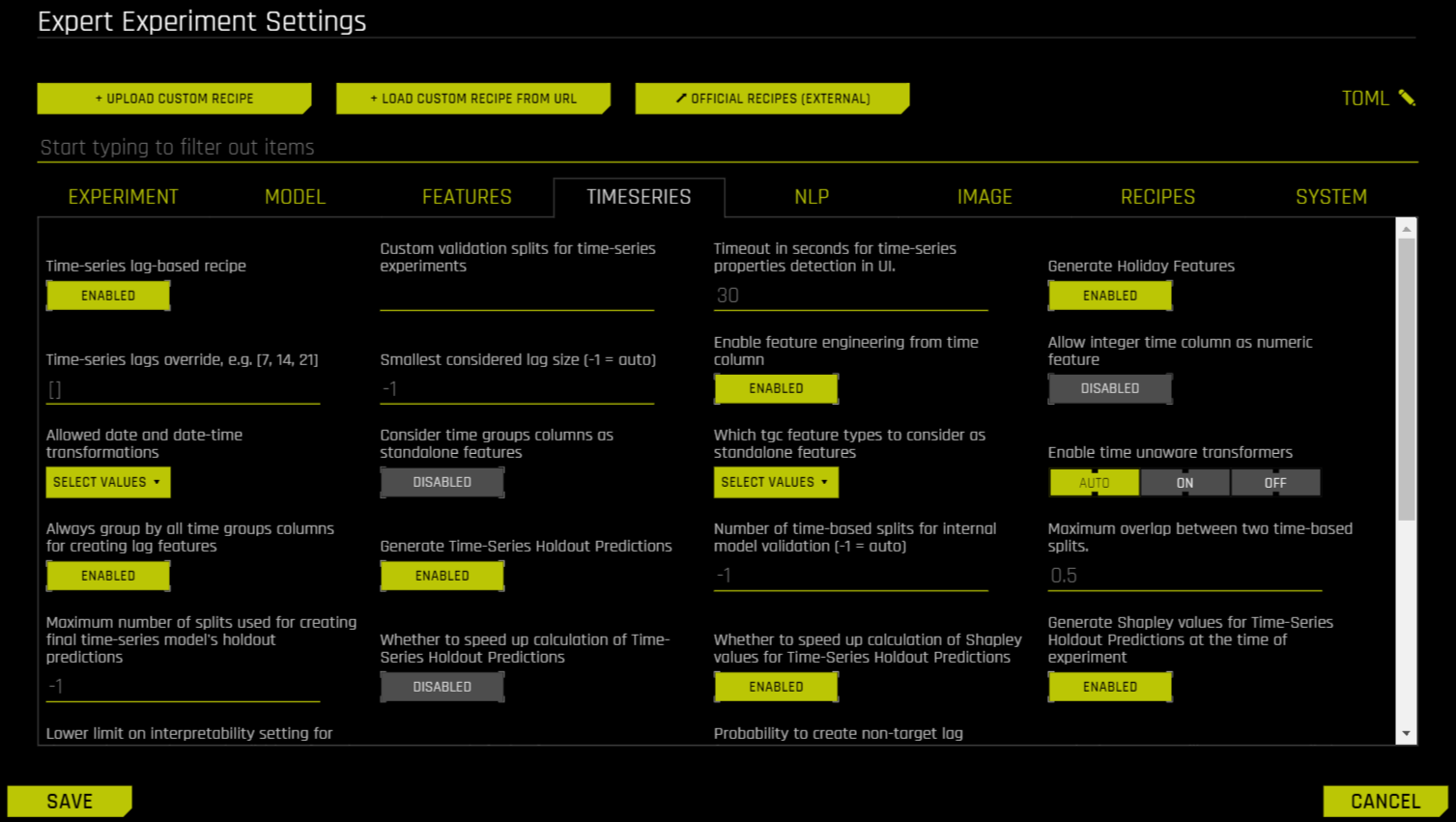
Time Series Expert Settings

The user may further configure the time series experiments with a dedicated set of options available through the Expert Settings panel. This panel is available from within the experiment page right above the Scorer knob.

Refer to Time Series Settings for more information on these options.

Time-series leaderboard mode

You can control the time-series leaderboard with the time_series_leaderboard_mode TOML config. Specify one of the following options:

• diverse: Explore a diverse set of models built using various expert settings. Note that you can rerun another diverse leaderboard on top of the best-performing model(s).

• sliding_window: If the forecast horizon is N periods, create a separate model for each of the (gap, horizon) pairs of (0,n), (n,n), (2*n,n), …, (2*N-1, n) in units of time periods. The number of periods to predict per model n is controlled by the expert setting time_series_leaderboard_periods_per_model, which defaults to 1.

Additional Resources

Refer to the following for examples showing how to run Time Series examples in Driverless AI:

• Time Series Best Practices

• Training a Time Series Model

• Time Series Recipes with Rolling Window

• Time Series Pipeline with Test Time Augmentation