Tutorial 1: Determine the model with the best robustness and stability
Overview
This tutorial explores how H2O Model Validation enables you to assess the robustness and stability of a set of models to determine the best model. In particular, we will assess two machine learning models to determine which one is more fit to achieve the purpose of the models, which is to predict house prices in Kansas City, Missouri.
Prerequisites
- Access to H2O Model Validation v0.17.0
- Ensure you turn on demo mode. See Turn on or off demo mode
- General knowledge of a size dependency test
- To learn more, see Size dependency
- General knowledge of a backtesting test
- To learn more, see Backtesting
- (Optional) Review Model Validation flow
Step 1: House prices models
For this tutorial, we will asses two machine learning models to determine which one is more fit to achieve the purpose of the model, which is to predict house prices in Kansas City. Let's begin.
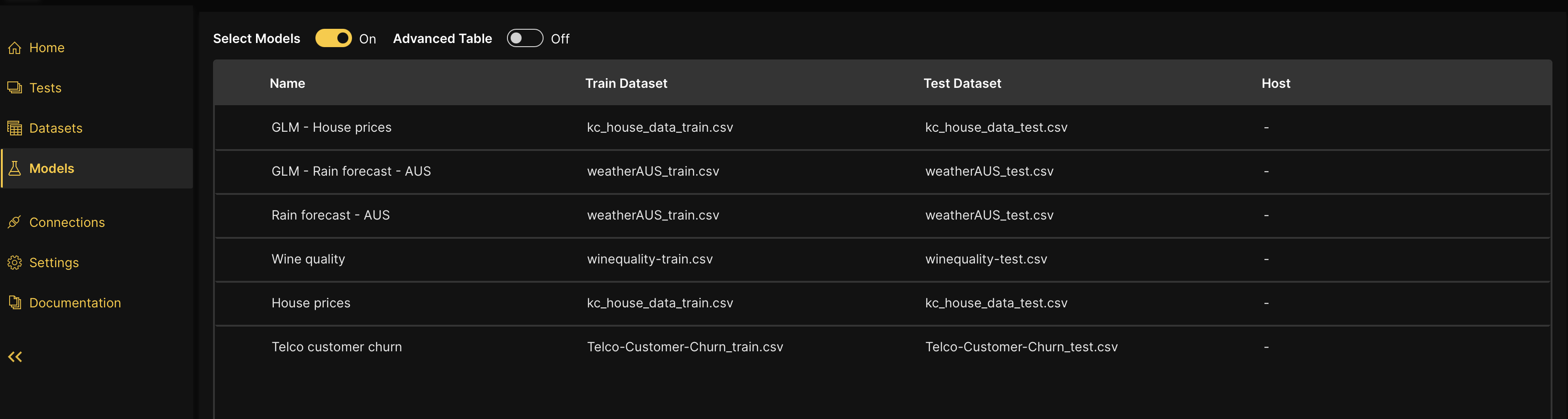
- In the H2O Model Validation navigation menu, click Models.
- In the Models table, please observe the following two models we will assess:
- GLM - House prices
- House prices
noteBoth models were trained to predict house prices in Kansas City. The main difference between both models is that the following is a generalized linear model (GLM): GLM - House prices.
Step 2: Compare models
Validation tests
H2O Model Validation supports an array of validation tests to assess the stability and robustness of a model. For purposes of this tutorial, we will utilize the following validation test types that have already been created for both models:
- Size dependency
- To learn how to create a size dependecy test for a model, see Create an adversarial similarity test.
- Backtesting
- To learn how to create a backtesting test for a model, see Create a backtesting test.
Let's compare the models. H2O Model Validation compares the models by comparing the associated validation tests with the models.
- Select the Select models toggle.
- Select the following two models to compare:
- GLM - House prices
- House prices

- Click Compare.
Comparison 1: Model summaries
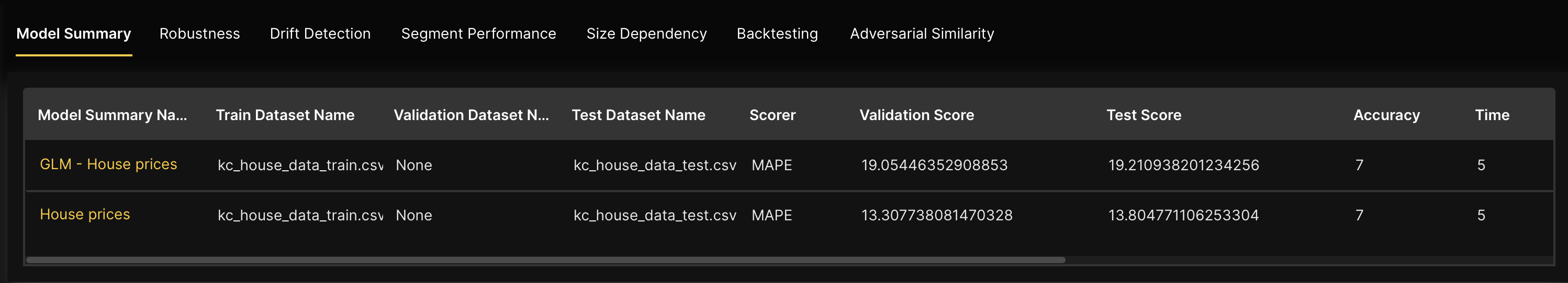
To start our comparison of both models, let's compare the models' validation and test scores. The scorer for both models is the mean absolute percentage error (MAPE). A lower MAPE will be considered good for our models.
In the Model summary table (in the Model summary tab), we see in the Validation score and Test score column that the non-GLM model received a lower MAPE.
Comparison 2: Size depedency
Now, let's compare the size dependency test of both models.
A size dependency test enables you to analyze the effects different sizes of train data will have on the accuracy of a selected model. In particular, size dependency facilitates model stability analysis and, for example, can answer whether augmenting an existing train data seems to be promising in terms of model accuracy. To learn more, see Size dependency.
- Click the Size dependency tab.
Left graph: The test MAPE scores graph displays the test MAPE values for the size dependency tests obtained with different test dataset sizes.
- X-axis: Train data sizes
- Y-axis: Test MAPE scores
Right graph: The validation MAPE scores graph displays the validation MAPE values for the size dependency tests obtained with different validation dataset sizes.
- X-axis: Train data sizes
- Y-axis: Validation MAPE scores
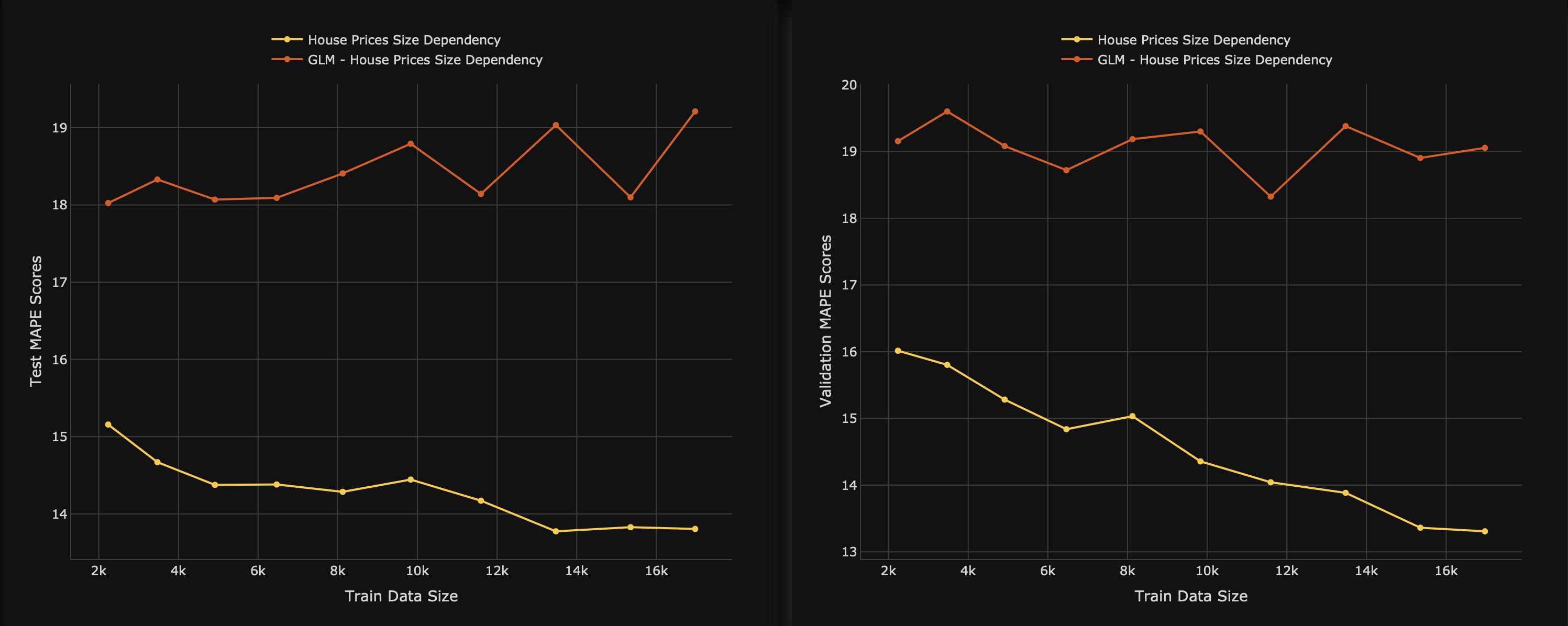
As we observe the size dependency graphs, we observe the following:
- The test and validation MAPE scores of the GLM model are higher with different sizes of data (orange line)
- The test and validation MAPE scores of the non-GLM model are lower with different sizes of data (yellow line)
Comparison 3: Backtesting
To conclude our comparison journey, let's compare the backtesting test of both models.
A backtesting test enables you to assess the robustness of a model by using the existing historical training data through a series of iterative training where training data is used from its recent to oldest collected values. To learn more, see Backtesting.
- Click the Backtesting tab.
Left graph: The test MAPE scores graph displays the back-test values for each split date of the backtesting tests, where back-test refers to the target distribution values of the backtesting test dataset.
- X-axis: Split dates
- Y-axis: Back-test MAPE scores
Right graph: The cross-validation MAPE scores graph displays the cross-validation values for each split date for the backtesting models. This graph can be helpful when estimating a model's fitness level to a dataset not used when training the model.
- X-axis: Split dates
- Y-axis: Cross-validation MAPE scores
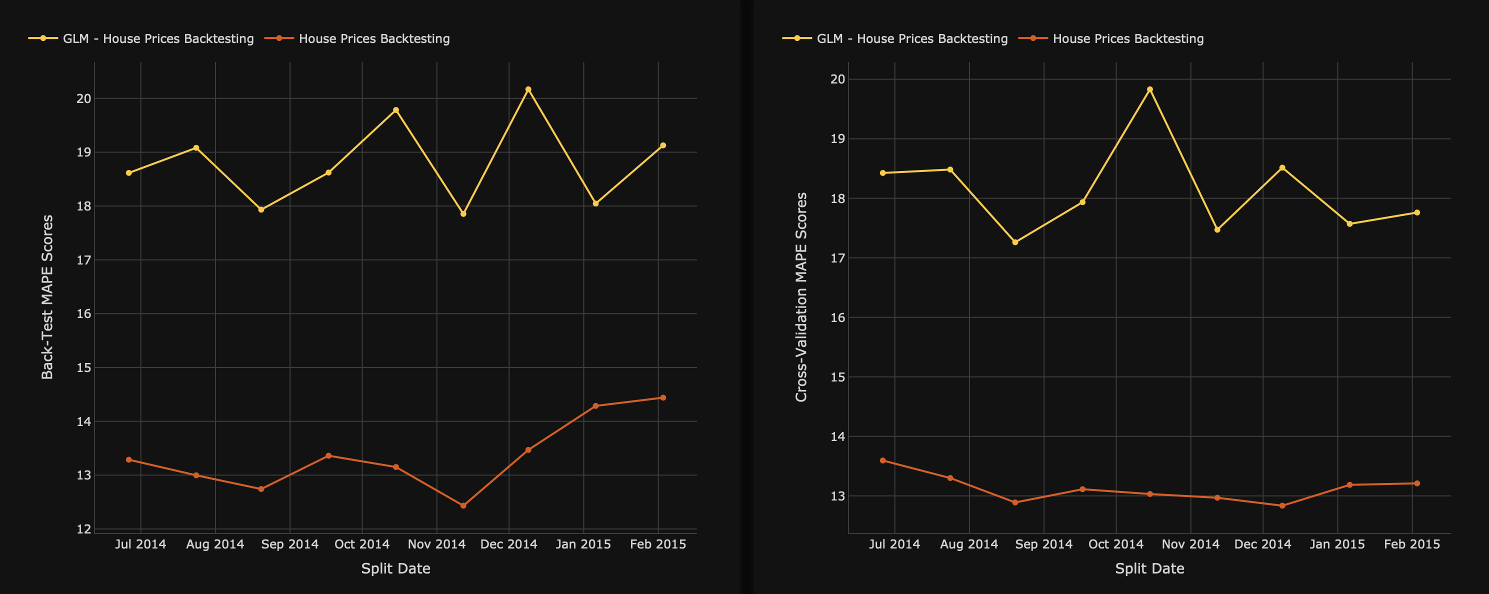
As we observe the backtesting graphs, we observe the following:
- The cross-validation and back-test MAPE scores of the GLM model vary at a higher frequency across the split dates. In other words, the variance of the model accuracy is not stable across time
- The cross-validation and back-test MAPE scores of the non-GLM model display a stable frequency across the split dates. In other words, it can be stated empirically that the variance of the model accuracy is stable across time
Step 3: Determine the best model (and the winner is...)
After comparing the two different house prices models, we can conclude that the non-GLM model is the more robust and stable to achieve the model's purpose (which is to predict house prices in Kansas City). Reasons being:
- According to the model summaries, the non-GLM model received a lower validation and test score.
- Based on the compared size dependency tests of the models, different sizes of train data have a low effect on the accuracy of the non-GLM model (in other words, the non-GLM model seems more stable).
- The non-GLM model shows more robustness when utilizing the existing historical training data. In other words, it can be stated empirically that the variance of the non-GLM model accuracy is more stable across time.
Summary
In this tutorial, we learned how H2O Model Validation enables you to assess the robustness and stability of a set of models to determine the best model.
- Submit and view feedback for this page
- Send feedback about H2O Model Validation to cloud-feedback@h2o.ai