Task 5: Diagnostics scores and confusion matrix
This task will focus on running a model diagnostic on the freddie_mac_500_test set. The diagnostics model allows you to view model performance for multiple scorers based on an existing model and dataset through the Python API.
Select DIAGNOSTICS on the tab above.
Once in the DIAGNOSTICS page, select + DIAGNOSE MODEL:
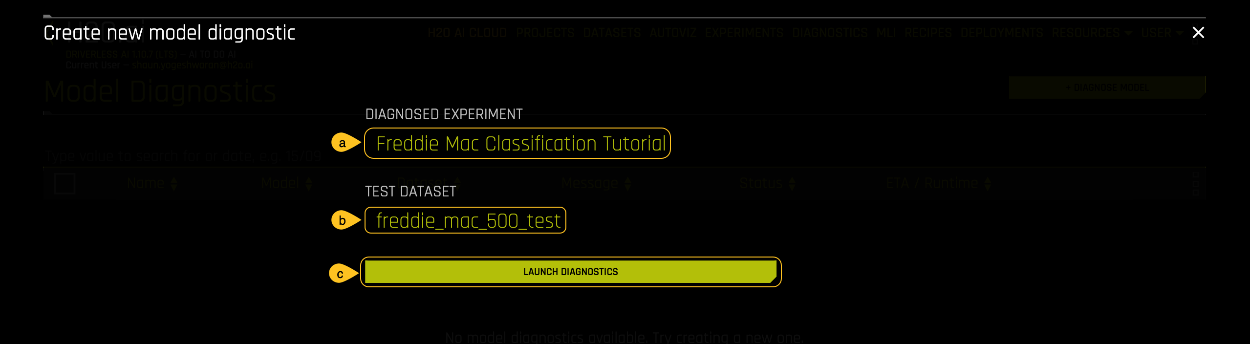
In the Create new model diagnostics section:
a. Click on Diagnosed Experiment then select the experiment that you completed in Task 4: Freddie Mac Classification Tutorial.
b. Click on Dataset then select the
freddie_mac_500_testdataset.c. Initiate the diagnostics model by clicking on LAUNCH DIAGNOSTICS.
After the model diagnostics is done running, a model similar to the one below will appear:
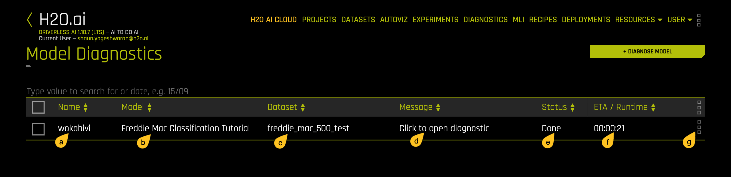
a. Name: Name of the new diagnostics model.
b. Model: Name of the ML model used for diagnostics.
c. Dataset: Mame of the dataset used for diagnostic.
d. Message : Message regarding the new diagnostics model.
e. Status : Status of the new diagnostics model.
f. ETA/Runtime : Time taken for the new diagnostics model to run.
g. Options for this model.
- Click on the new diagnostics model and a page similar to the one below will appear:
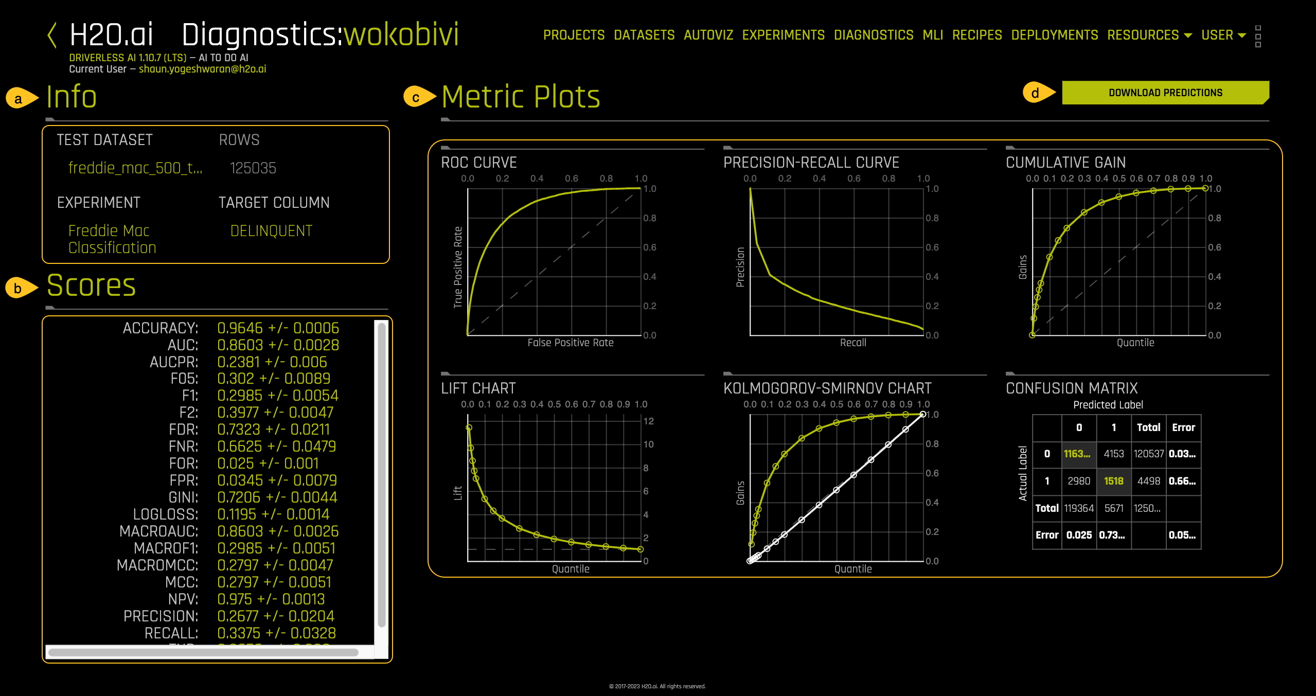
a. Info: Information about the diagnostics model including the name of the test dataset, name of the experiment used, and the target column used for the experiment.
b. Scores: Summary for the values for GINI, MCC, F05, F1, F2, Accuracy, Log loss, AUC and AUCPR in relation to how well the experiment model scored against a “new” dataset.
c. Metric Plots: Metrics used to score the experiment model including ROC Curve, Pre-Recall Curve, Cumulative Gains, Lift Chart, Kolmogorov-Smirnov Chart, and Confusion Matrix.
d. DOWNLOAD PREDICTIONS: Download the diagnostics predictions.
- The new dataset must be the same format and with the same number of columns as the training dataset.
- The scores will be different for the train dataset and the validation dataset used during the training of the model.
Confusion matrix
The confusion matrix, also known as the error matrix, is the foundation for most metrics used to evaluate a supervised model's classification performance, including its error rate. This table allows you to calculate various metrics, such as error rate, accuracy, specificity, sensitivity, and precision. These metrics provide insights into how well your model performs at classifying or predicting data points.
Click on the CONFUSION MATRIX plot located under the Metrics Plot section of the DIAGNOSTICS page.
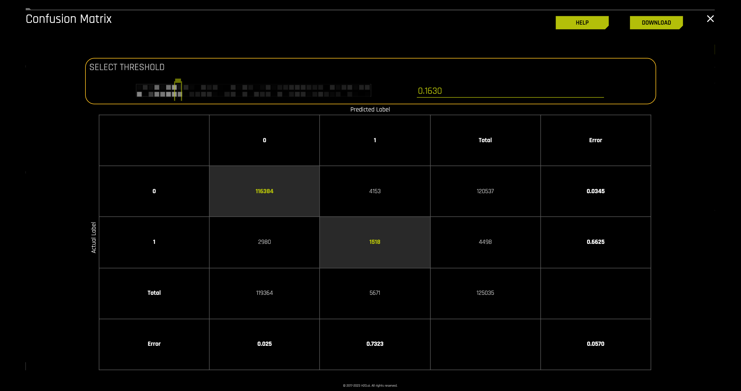
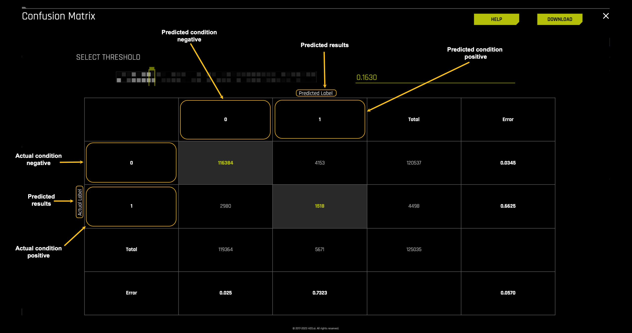
The confusion matrix lets you choose the desired threshold for your predictions. In this case, we will take a closer look at the confusion matrix generated by the Driverless AI model with the default threshold, which is 0.1630.
The first part of the confusion matrix we will look at is the Predicted labels and the Actual labels. As shown on the image below the Predicted label values for Predicted Condition Negative or 0 and Predicted Condition Positive or 1 run vertically while the Actual label values for Actual Condition Negative or 0 and Actual Condition Positive or 1 run horizontally on the matrix.
Using this layout, we will determine how well the model predicted the people that defaulted and those that did not from our Freddie Mac test dataset. Additionally, we will be able to compare it to the actual labels from the test dataset.
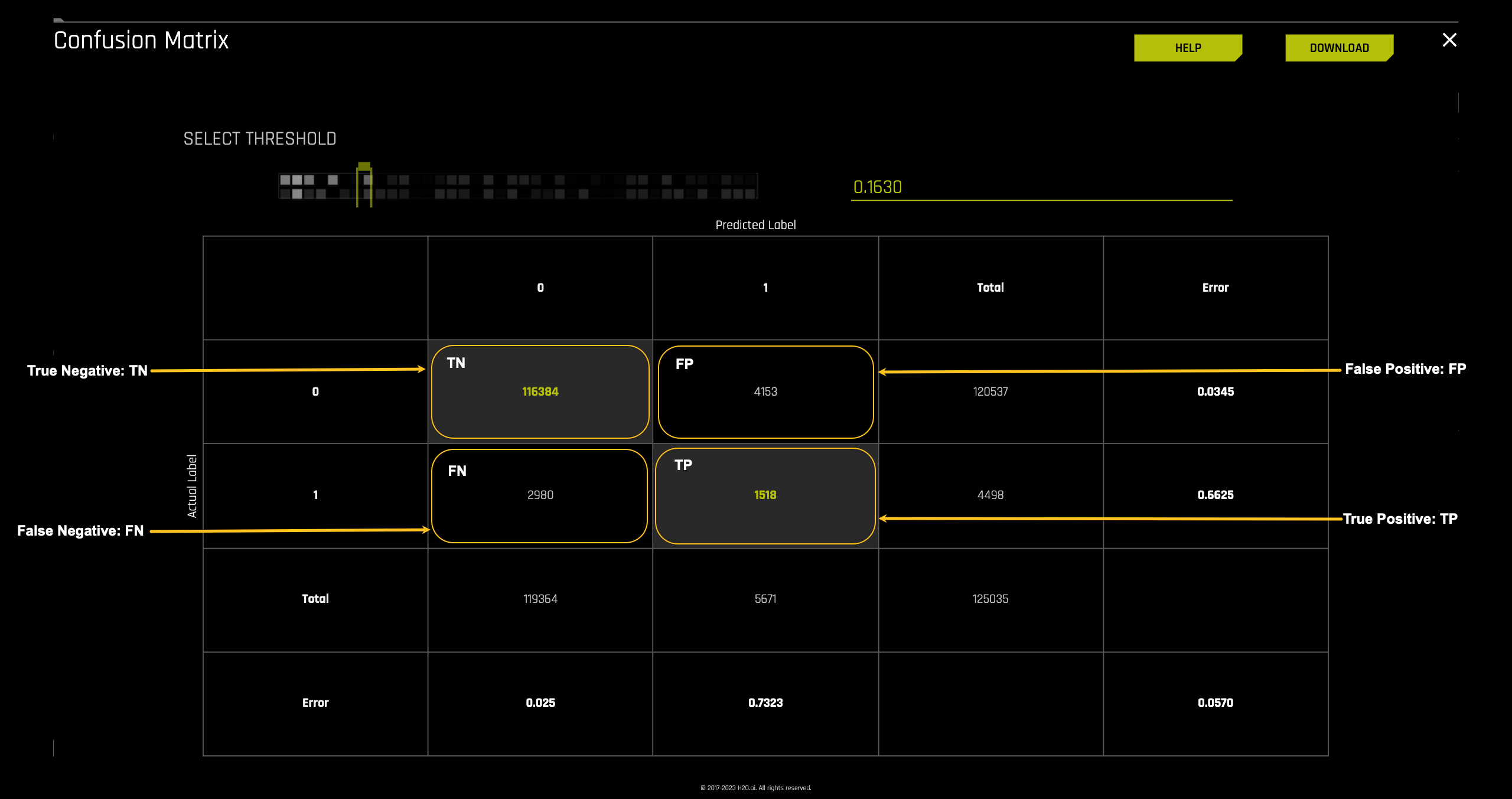
Moving into the matrix's inner part, we find the number of cases for True Negatives, False Positives, False Negatives, and True Positives. The confusion matrix for this model generated tells us that:
- TP = 1,518 cases were predicted as defaulting and defaulted in actuality
- TN = 116,384 cases were predicted as not defaulting and did not default
- FP = 4,153 cases were predicted as defaulting when in actuality they did not default
- FN = 2,980 cases were predicted as not defaulting when in actuality they defaulted
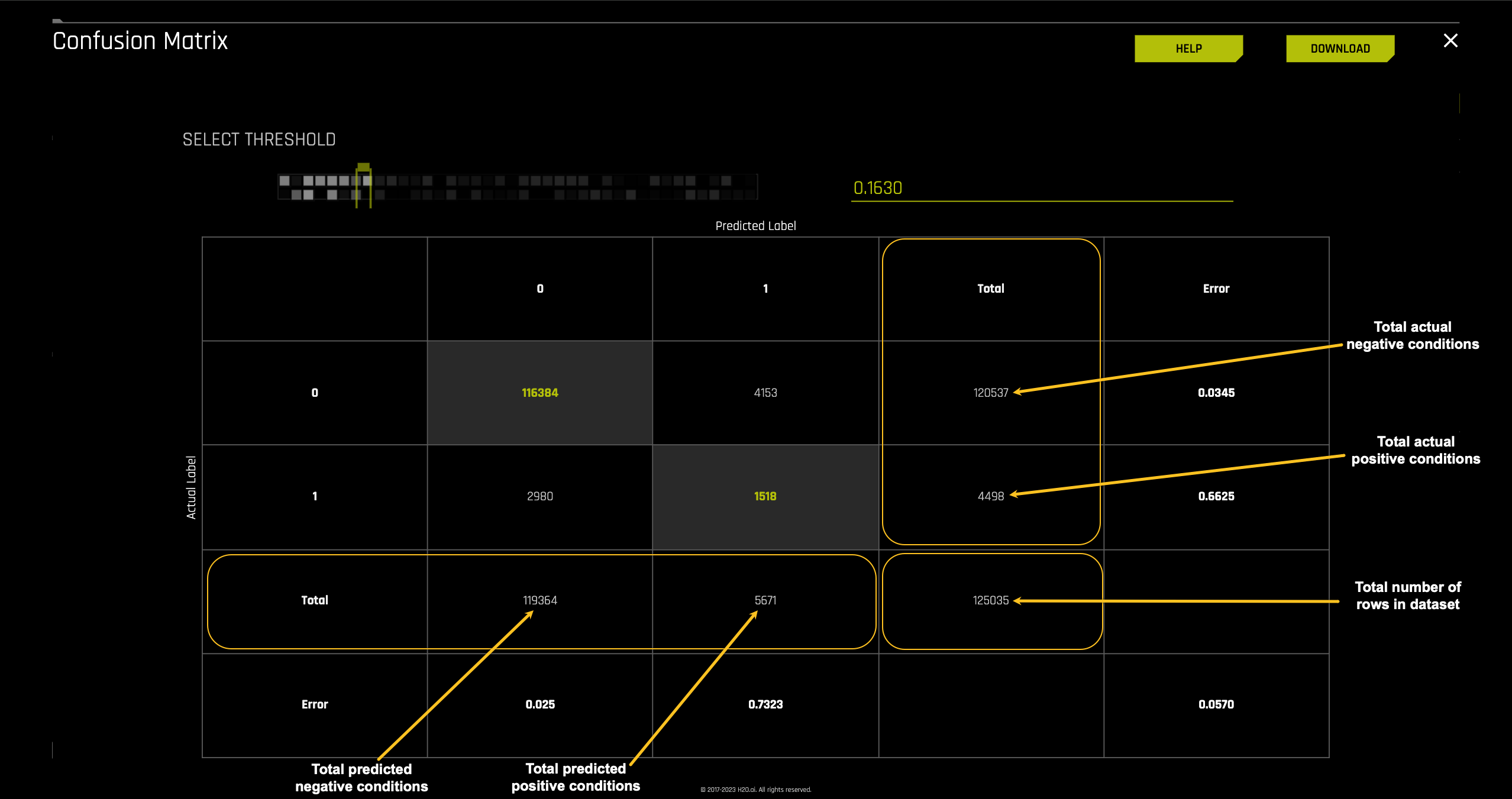
The next layer we will look at is the Total sections for Predicted label and Actual label.
On the right side of the confusion matrix are the totals for the Actual label and at the base of the confusion matrix, the totals for the Predicted label.
Actual label
- 120,537: the number of actual cases that did not default on the test dataset
- 4,498: the number of actual cases that defaulted on the test
Predicted label
- 119,364: the number of cases that were predicted to not default on the test dataset
- 5,671: the number of cases that were predicted to default on the test dataset
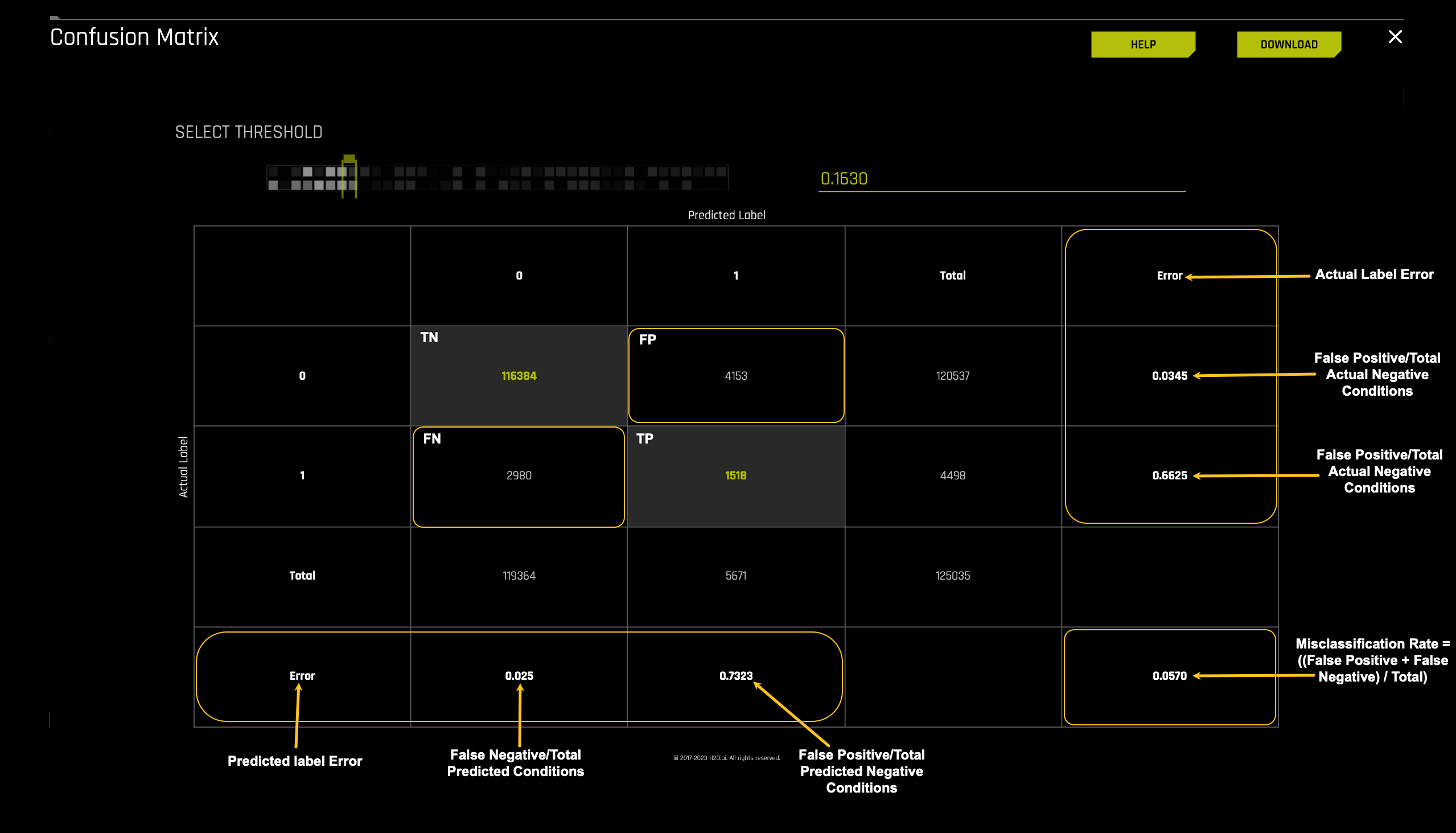
The final layer of the confusion matrix we will explore is the errors. The errors section is one of the first places where we can check how well the model performed. The better the model does at classifying labels on the test dataset, the lower the error rate. The error rate, also known as the misclassification rate, answers how often the model is wrong.
For this particular model these are the errors:
- 4153/120537 = 0.0344 or 3.4% times the model classified actual cases that did not default as defaulting out of the actual non-defaulting group
- 2980/4498 = 0.6625 or 66.3% times the model classified actual cases that did default as not defaulting out of the actual defaulting group
- 2980/119364 = 0.0249 or 2.49% times the model classified predicted cases that did default as not defaulting out of the total predicted not defaulting group
- 1518/5671 = 0.2676 or 26.76% times the model classified predicted cases that defaulted as defaulting out of the total predicted defaulting group
- (2980 + 4153) / 125035 = 0.0570 This means that this model incorrectly classifies 0.0570 or 5.7% of the time.
Interpreting the misclassification error 0.0570:
- The misclassification error of 0.0570 indicates that the model incorrectly classified 5.7% of the cases.
One way to look at the financial implications for Freddie Mac is to look at the total paid interest rate per loan. The mortgages on this dataset are traditional home equity loans which means that the loans are:
- A fixed borrowed amount
- Fixed interest rate
- Loan term and monthly payments are both fixed
For this tutorial, we will assume a 6% Annual Percent Rate (APR) over 30 years. APR is the amount one pays to borrow the funds. Additionally, we are going to assume an average home loan of $167,473 (this average was calculated by taking the sum of all the loans on the freddie_mac_500.csv dataset and dividing it by 30,001 which is the total number of mortgages on this dataset). For a mortgage of $167,473 the total interest paid after 30 years would be $143,739.01.
When looking at the False Positives, we can think about 4153 cases of people that the model predicted should not be granted a home loan because they were predicted to default on their mortgage. These 4153 loans translate to over 596 million dollars in loss of potential income (5147 * $143,739.01) in interest.
Looking at the False Negatives, we do the same and take the 2980 cases that were granted a loan because the model predicted that they would not default on their home loan. These 2980 cases translate to about over 428 million dollars in interest losses since 2794 in actuality cases defaulted.
The misclassification rate provides a summary of the sum of the False Positives and False Negatives divided by the total cases in the test dataset. The misclassification rate for this model was 0.0570. If this model were used to determine home loan approvals, the mortgage institutions would need to consider approximately 428 million dollars in losses for misclassified loans that got approved and shouldn’t have. Also, 596 million dollars on loans that were not approved since they were classified as defaulting.
This model helps decide whether to approve loans. But there's a trade-off to consider:
- Missed Opportunities: The model might reject good loans (false negatives), costing an estimated 596 million dollars.
- Losses from Defaults: The model might approve loans that later default (false positives), leading to actual losses of 428 million dollars so far.
The best approach depends on what the mortgage company values more:
- Avoiding defaults (even if it means missing some good loans)
- Approving more loans (even if it means some defaults)
- By considering these costs, the company can make informed decisions about using the model.
Scores
Driverless AI conveniently provides a summary of the scores for the performance of the model given the test dataset.
The scores section provides a summary of the Best Scores found in the metrics plots:
- ACCURACY
- AUC
- AUCPR
- F05
- F1
- F2
- FDR
- FNR
- FOR
- FPR
- GINI
- LOGLOSS
- MACROAUC
- MCC
- NPV
- PRECISION
- RECALL
- TNR
The image below represents the scores for the Freddie Mac Classification Tutorial model using the freddie_mac_500_test dataset:
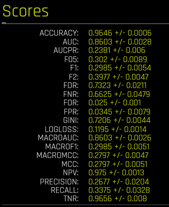
When we ran the experiment for this classification model, Driverless AI determined that the best scorer for it was the Logarithmic Loss or LOGLOSS due to the dataset's imbalanced nature. LOGLOSS focuses on getting the probabilities right (strongly penalizes wrong probabilities). The selection of Logarithmic Loss makes sense since we want a model that can correctly classify those who are most likely to default while ensuring that those who qualify for a loan can get one.
Recall that Log loss is the logarithmic loss metric that can be used to evaluate the performance of a binomial or multinomial classifier, where a model with a Log loss of 0 would be the perfect classifier. Our model scored a LOGLOSS value = 0.1195+/- 0.0014 after testing it with test dataset. From the confusion matrix, we saw that the model had issues classifying perfectly; however, it was able to classify with an ACCURACY of 0.9646 +/- 0.0006. The financial implications of the misclassifications have been covered in the confusion matrix section above.
Driverless AI has the option to change the type of scorer used for the experiment. Recall that for this dataset, Driverless AI selected LOGLOSS as the scorer. An experiment can be re-run with another scorer. For general imbalanced classification problems, AUCPR and MCC scorers are good choices, while F05, F1, and F2 are designed to balance recall and precision. The AUC is designed for ranking problems. Gini is similar to the AUC but measures the quality of ranking (inequality) for regression problems.
Congratulations, you now know how to run a model diagnostic on a dataset view model performance for multiple scorers. The next tutorial will focus on the financial implications of misclassification by exploring the confusion matrix and plots derived from it.
- Submit and view feedback for this page
- Send feedback about H2O Driverless AI | Tutorials to cloud-feedback@h2o.ai