Task 6: ER: ROC
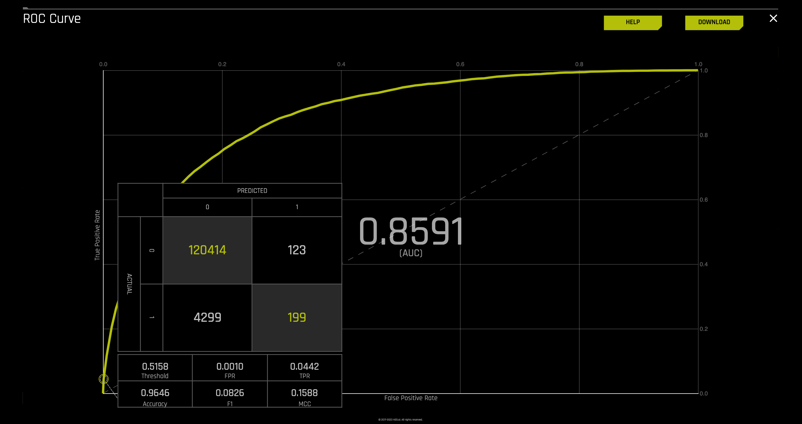
From the Diagnostics page, click on the ROC CURVE. THe ROC curve should look similar to the one below:
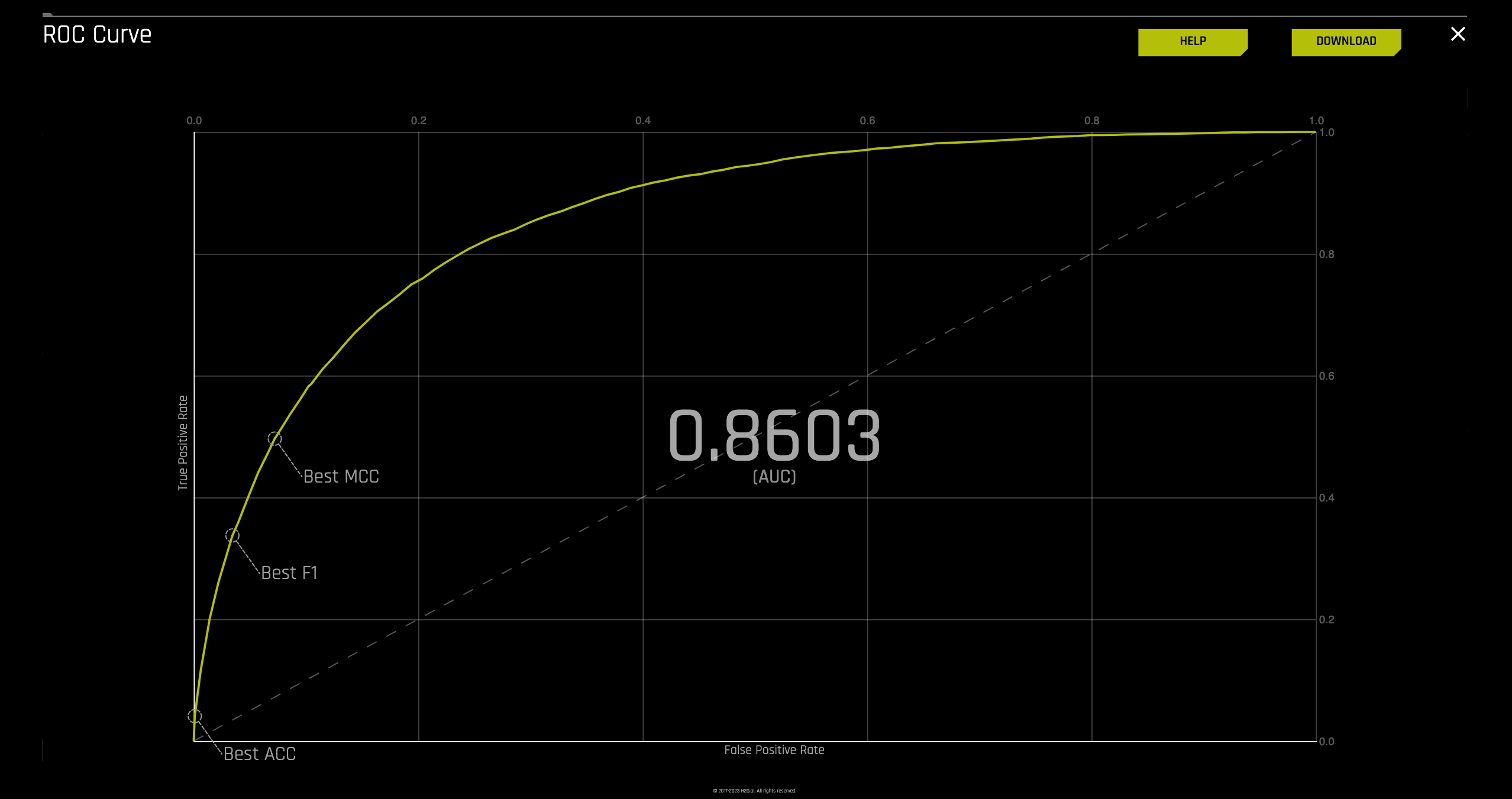
The ROC curve demonstrates the following:
- It shows the tradeoff between sensitivity (True Positive Rate or TPR) and specificity (1-FPR or False Positive Rate). A decrease in specificity will accompany any increase in sensitivity.
- The closer the curve follows the upper-left-hand border of the ROC space, the more accurate the model.
- The closer the curve comes to the 45-degree diagonal of the ROC space, the less accurate the model.
- The slope of the tangent line at a cutpoint gives the likelihood ratio (LR) for the test's value. You can check this out on the graph above.
- The area under the curve is a measure of model accuracy.
Returning to the Freddie Mac dataset, the model was evaluated using Logarithmic Loss to penalize errors. However, we can also examine the ROC curve to see if it aligns with our conclusions from the confusion matrix and scores in the diagnostics page.
From the ROC curve generated by Driverless AI for your experiment, identify the Area Under the Curve (AUC). Note that a perfect classification model achieves an AUC of 1.
For each point on the curve below, hover over it to determine the True Positive Rate (TPR), False Positive Rate (FPR), and corresponding threshold.
- Best Accuracy
- Best F1
- Best MCC
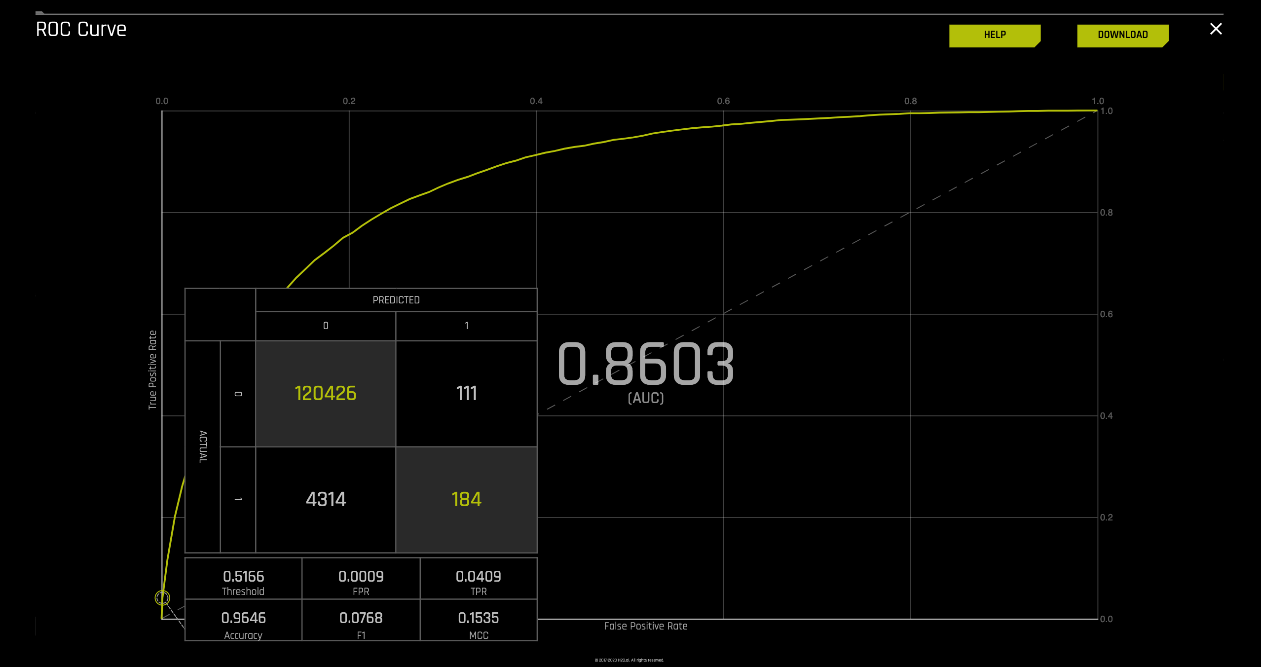
Recall that for a binary classification problem, accuracy is the number of correct predictions made as a ratio of all predictions made. Probabilities are converted to predicted classes to define a threshold. This model determined that the best accuracy is found at threshold 0.5166.
At this threshold, the model predicted:
- TP = 184 cases predicted as defaulting and defaulted.
- TN = 120,426 cases predicted as not defaulting and did not default.
- FP = 111 cases predicted as defaulting and did not default.
- FN = 4,314 cases predicted to not default and defaulted.
- Use the key points below to help you assess the ROC Curve:
- The perfect classification model has an AUC of 1
- MCC is measured in the range between -1 and +1 where +1 is the perfect prediction, 0 no better than a random prediction, and -1 being all incorrect predictions.
- F1 is measured in the range of 0 to 1, where 0 means that there are no true positives, and 1 when there is neither false negatives nor false positives or perfect precision and recall.
- Accuracy is measured in the range of 0 to 1, where 1 is perfect accuracy or perfect classification, and 0 is poor accuracy or poor classification.
If you are not sure what AUC, MCC, F1, and Accuracy are or how they are calculated review the concepts section of this tutorial.
New experiment with same settings
In case you wanted to know if you could improve the accuracy of the model, you can try changing the scorer from Logloss to Accuracy.
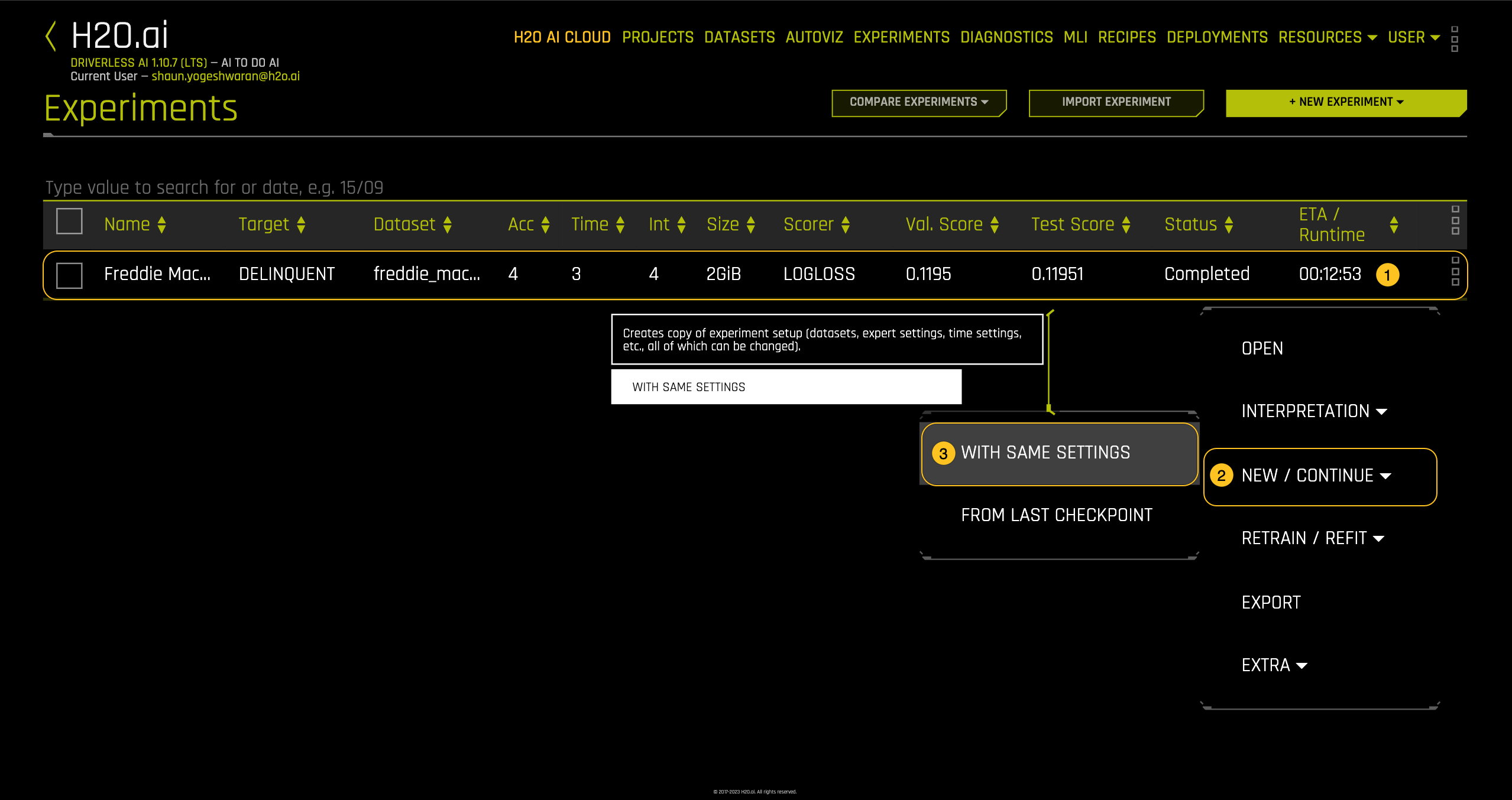
To do this, click on the Experiments page.
Click on the experiment you did for task 1 and select NEW/CONTINUE and then WITH SAME SETTINGS:
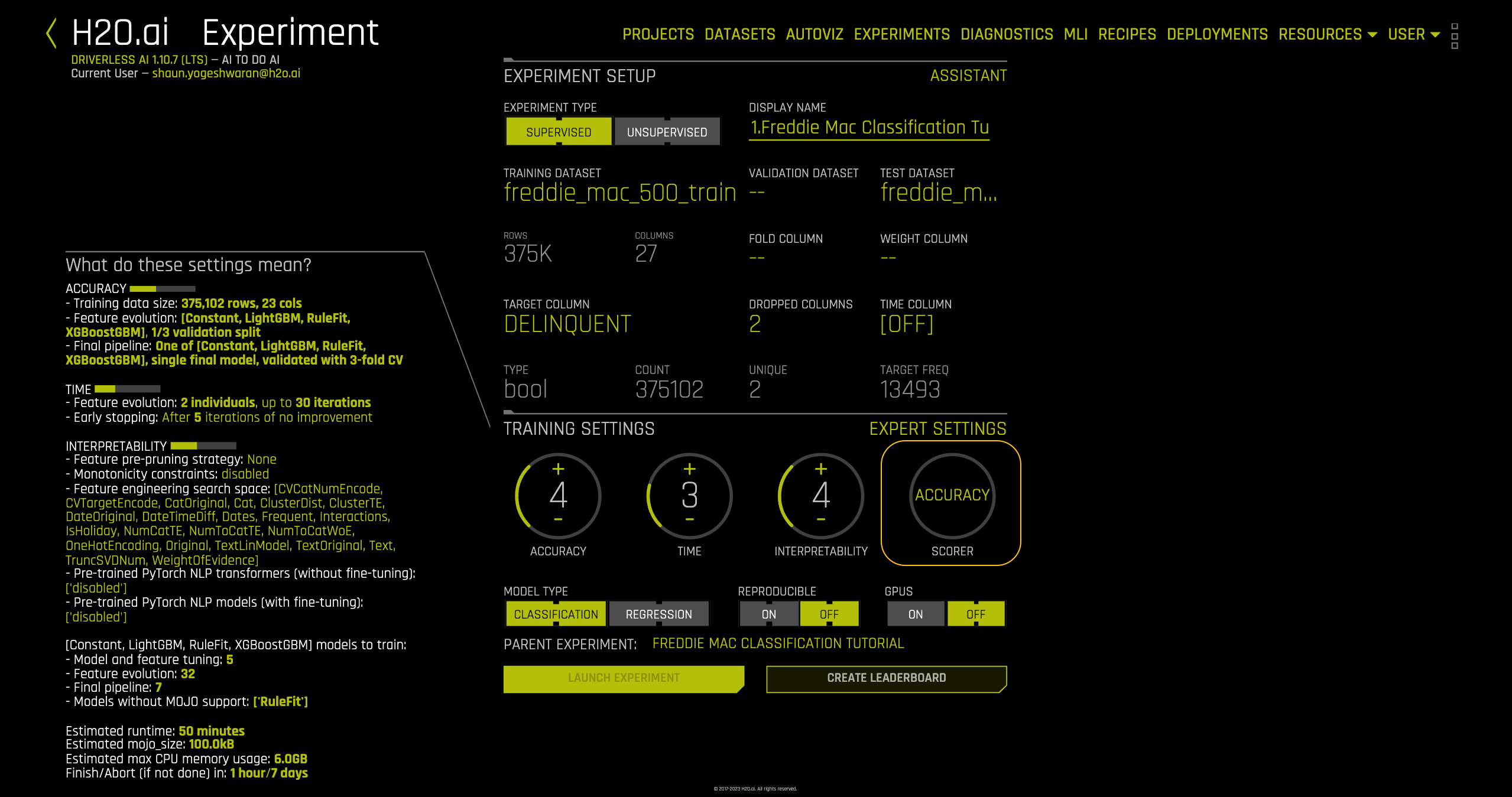
 An image similar to the one above will appear. Note that this page has the same settings as the setting in Task 1. The only difference is that on the Scorer section, we updated Logloss to Accuracy. Everything else will remain the same.
If you haven’t done so, select ACCURACY on the scorer section then select LAUNCH EXPERIMENT:
Similarly to the experiment in Task 1, wait for the experiment to run. After the experiment is done running, a similar page will appear. Note that on the summary located on the bottom right-side, both the validation and test scores are no longer being scored by LOGLOSS instead by ACCURACY.
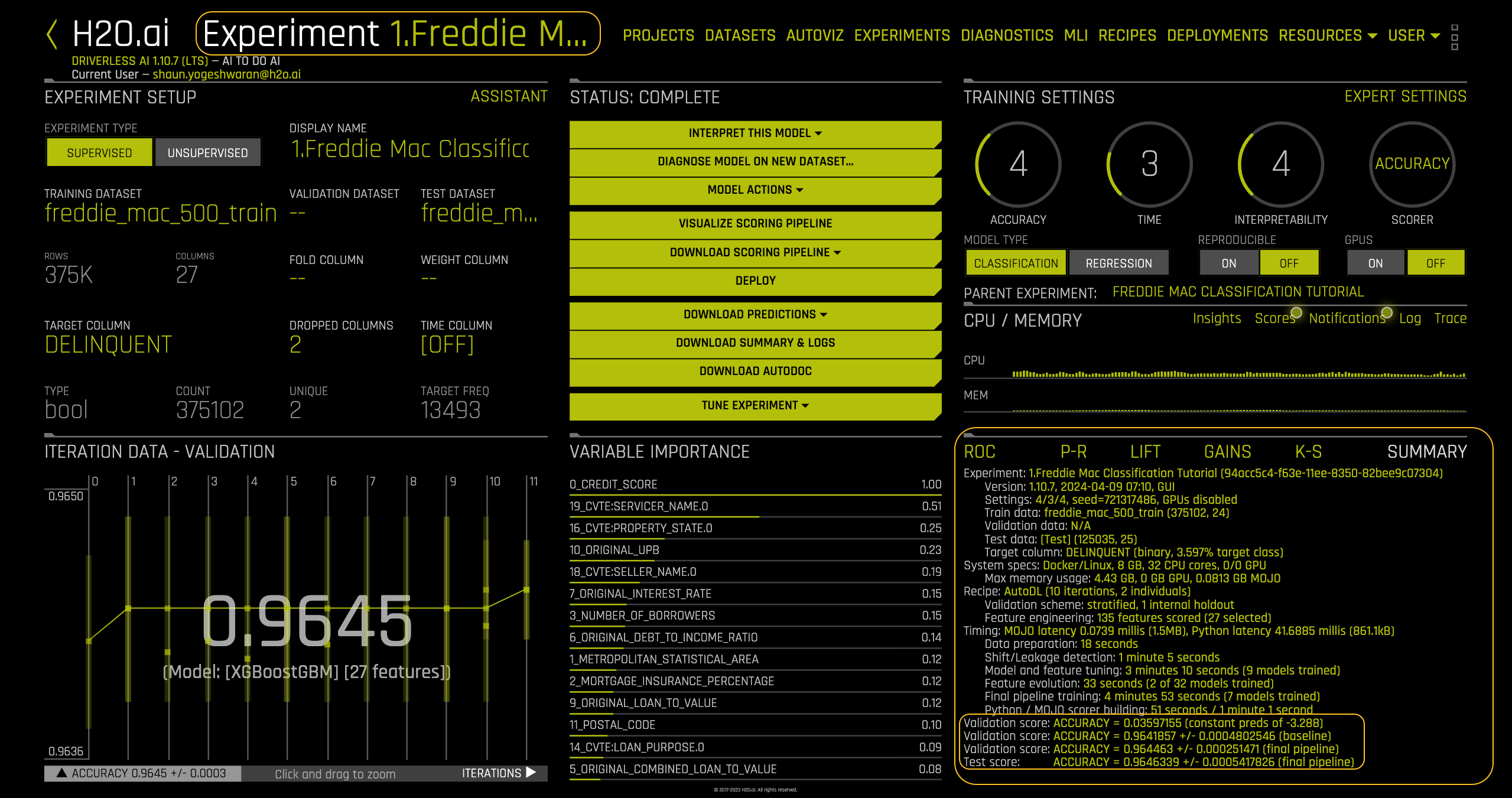
We are going to use this new experiment to run a new diagnostics test. You will need the name of the new experiment. In this case, the experiment name is 1.Freddie Mac Classification Tutorial.
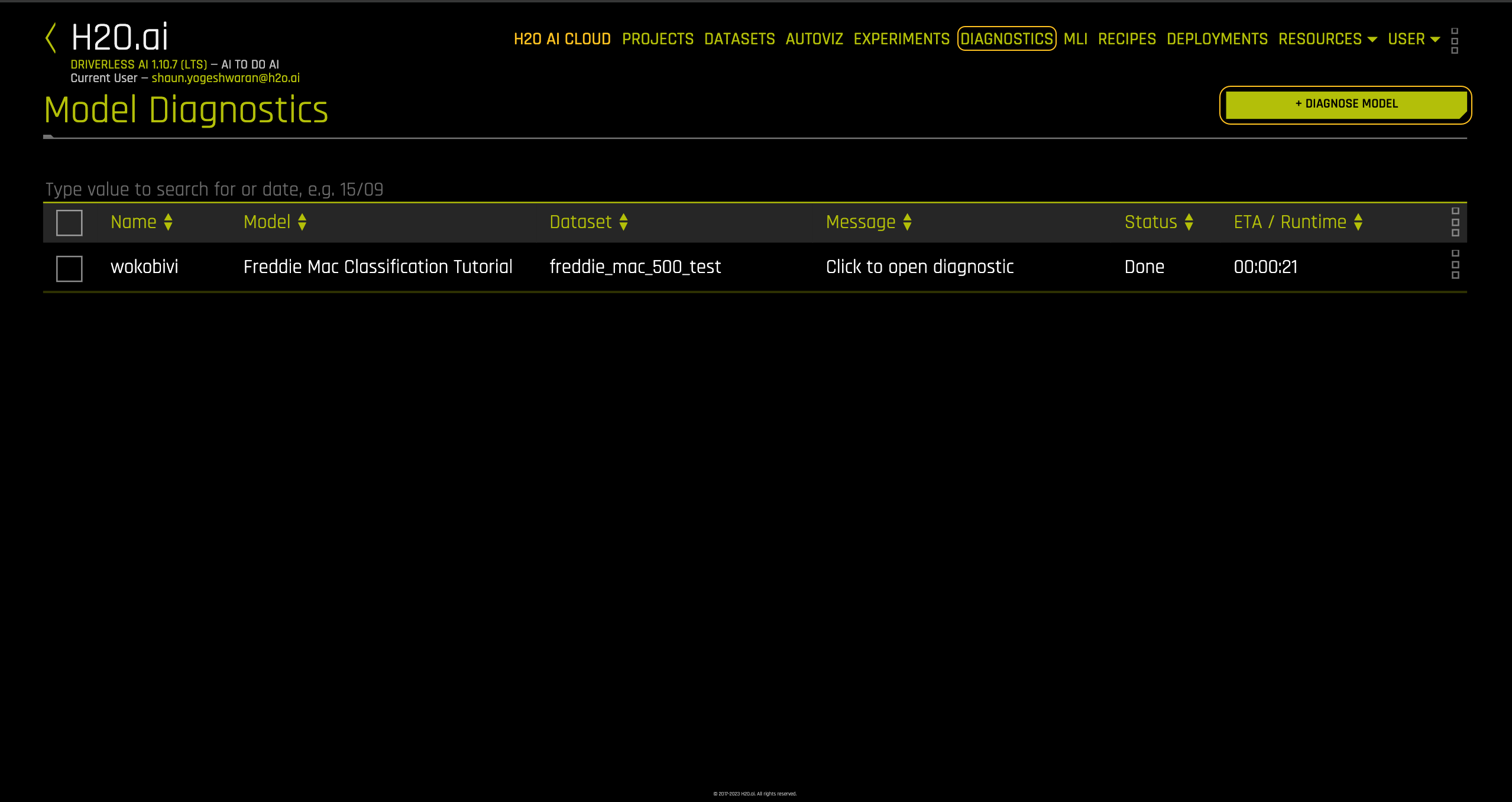
Go to the DIAGNOSTICS tab.
Once in the DIAGNOSTICS page, select +DIAGNOSE MODEL.
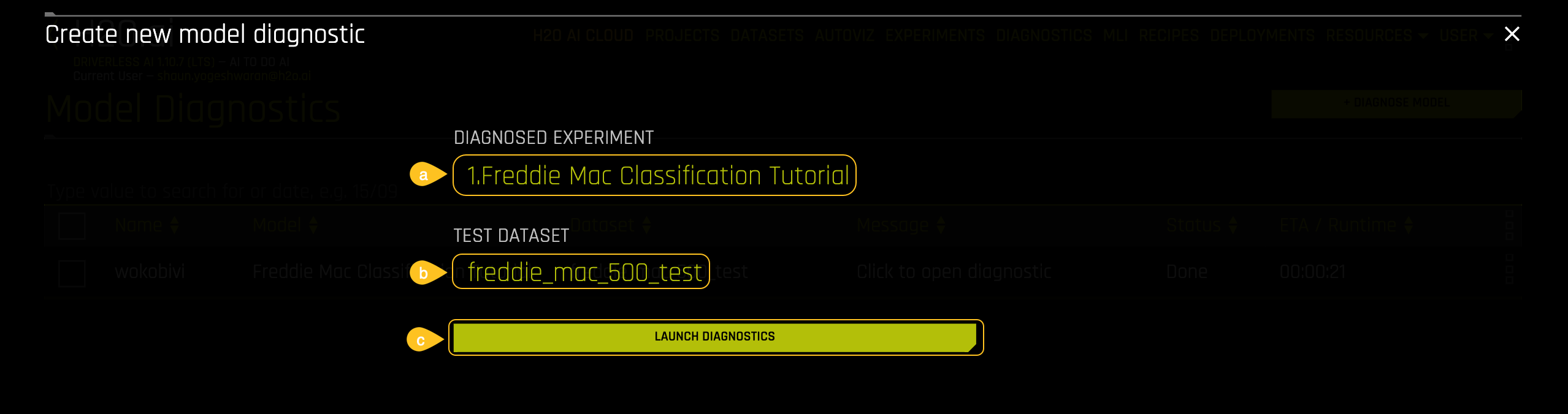
In the Create new model diagnostics:
a. Click on DIAGNOSED EXPERIMENT, then select the experiment that you completed in this Task. In this case, the experiment name is 1.Freddie Mac Classification Tutorial.
b. Click on TEST DATASET then select the freddie_mac_500_test dataset.
c. Initiate the diagnostics model by clicking on LAUNCH DIAGNOSTICS:
After the model diagnostics is done running, a new diagnostic will appear.
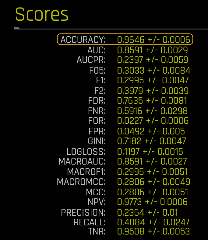
Click on the new diagnostics model. On the Scores section, observe the accuracy value.
- Next, locate the new ROC curve and click on it. Hover over the Best ACC point on the curve.
Impact of Optimized Threshold on Model Performance.
This section analyzes the effect of optimizing the model's decision threshold on classification performance. The evaluation is based on a confusion matrix comparing the original and the new model's performance.
The first model predicted:
- Threshold = 0.5166
- TP = 184 cases predicted as defaulting and defaulted
- TN = 120,426 cases predicted as not defaulting and did not default
- FP = 111 cases predicted as defaulting and did not default
- FN = 4,314 cases predicted to not default and defaulted
The new model predicted:
- Threshold = 0.5158
- TP = 199 cases predicted as defaulting and defaulted
- TN = 120,414 cases predicted as not defaulting and did not default
- FP = 123 cases predicted as defaulting and did not default
- FN = 4,299 cases predicted not to default and defaulted
| Metric | Original Model (Threshold: 0.5166) | New Model (Threshold: 0.5158) |
|---|---|---|
| True Positives (TP) | 184 | 199 |
| True Negatives (TN) | 120426 | 120414 |
| False Positives (FP) | 111 | 123 |
| False Negatives (FN) | 4314 | 4299 |
The threshold for optimal accuracy has been adjusted from 0.5166 in the initial diagnostics model to 0.5158 in the updated model. This alteration in threshold has impacted the accuracy of correct predictions relative to all predictions. While there has been a decrease in false positives (FPs), there has also been an increase in false negatives (FNs). Our efforts led to a reduction in cases predicted to falsely default, but this resulted in an increase in cases predicted not to default which defaulted.
The key insight is that achieving a perfect balance is challenging; trade-offs are inevitable. In pursuit of accuracy, we reduced the instances of mortgage loans, particularly for individuals denied mortgages due to erroneous default predictions. However, we also increased instances where loans were granted to individuals who should not have qualified.
- Exit out of the ROC curve by clicking on the X located at the top-right corner of the plot, next to the DOWNLOAD option
This task has provided you with a deeper understanding of the ROC curve and how to optimize the model's threshold to improve classification performance. The next task will focus on the Prec-Recall curve.
- Submit and view feedback for this page
- Send feedback about H2O Driverless AI | Tutorials to cloud-feedback@h2o.ai