Version: v1.1.0

Analyze drift in Superset

Before you begin

Before running drift queries, ensure the following:

Your deployment is Healthy and actively scoring requests. See Configure monitoring for setup instructions.
At least 3–5 minutes have elapsed after the first scoring request, to allow aggregation data to populate.
You have workspace access for the deployment you want to analyze. Users can only query schemas for workspaces they have access to.

Drift detection methods

The following table summarizes the available drift detection methods. These are examples; the appropriate method depends on your data and use case.

Method	Feature type	Use case	Key metric
TVD (Total Variation Distance)	Numerical	General-purpose drift detection for numerical features	0 (identical) to 1 (completely different)
TVD with time window aggregation	Numerical	Drift detection with configurable time buckets for small samples	Aggregates across time windows before calculating
PSI (Population Stability Index)	Categorical	Drift detection for categorical features using value counts	< 0.10 no drift, > 0.25 significant drift
Z-Score	Numerical	Quick mean-shift detection using standard deviations	Number of standard deviations from baseline
Hellinger Distance	Numerical	Distribution overlap comparison (minute-level only)	0 (identical) to 1 (no overlap)

Choosing the right drift method

For numerical features with sufficient data: Use TVD for a straightforward drift score.
For numerical features with small samples: Use TVD with time window aggregation to aggregate across time windows before calculating drift.
For categorical features: Use PSI to detect drift in categorical features using probability shifts.
For a quick mean-shift check: Use Z-Score with configurable time windows.
For distribution overlap analysis at minute granularity: Use Hellinger Distance.

Running drift queries

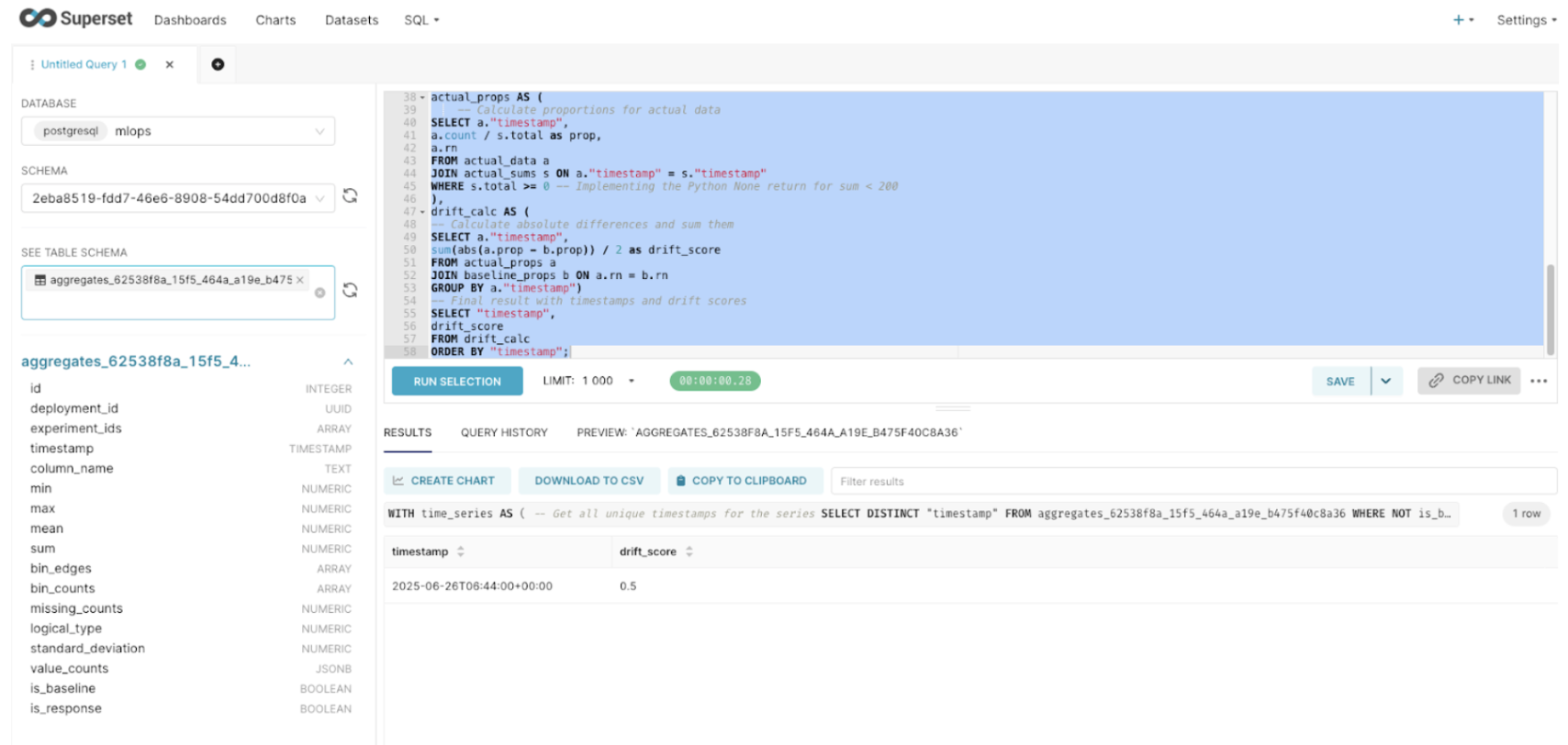
In Superset SQL Lab, replace <TABLE_NAME> with your aggregates_<deployment_id> table and <FEATURE_NAME> with the column name you want to analyze (e.g., 'AGE').

Drift query

TVD numerical drift

Total Variation Distance (TVD) measures the overall difference between the baseline and actual data distributions by computing half the sum of absolute differences between probability distributions. Values range from 0 (identical distributions) to 1 (completely different distributions).

WITH time_series AS (
-- Get all unique timestamps for the series
SELECT DISTINCT "timestamp"
FROM <TABLE_NAME>
WHERE NOT is_baseline
AND column_name = <FEATURE_NAME>
ORDER BY "timestamp"),
baseline AS (
-- Get the baseline (expected) data
SELECT unnest(bin_counts) as count
FROM <TABLE_NAME>
WHERE is_baseline
AND column_name = <FEATURE_NAME>),
baseline_sum AS (
-- Calculate sum of baseline counts
SELECT sum(count) as total
FROM baseline),
baseline_props AS (
-- Calculate baseline proportions
SELECT count / total        as prop,
row_number() OVER () as rn
FROM baseline,
baseline_sum),
actual_data AS (
-- Get actual data for each timestamp
SELECT "timestamp",
unnest(bin_counts)                            as count,
row_number() OVER (PARTITION BY "timestamp") as rn
FROM <TABLE_NAME>
WHERE NOT is_baseline
AND column_name = <FEATURE_NAME>),
actual_sums AS (
-- Calculate sums for each timestamp
SELECT "timestamp",
sum(count) as total
FROM actual_data
GROUP BY "timestamp"),
actual_props AS (
-- Calculate proportions for actual data
SELECT a."timestamp",
a.count / s.total as prop,
a.rn
FROM actual_data a
JOIN actual_sums s ON a."timestamp" = s."timestamp"
WHERE s.total >= 0
),
drift_calc AS (
-- Calculate absolute differences and sum them
SELECT a."timestamp",
sum(abs(a.prop - b.prop)) / 2 as drift_score
FROM actual_props a
JOIN baseline_props b ON a.rn = b.rn
GROUP BY a."timestamp")
-- Final result with timestamps and drift scores
SELECT "timestamp",
drift_score
FROM drift_calc
ORDER BY "timestamp";

TVD with time window aggregation

This query aggregates bin counts across configurable time windows before calculating drift. This is recommended when you have a small number of scoring requests, as it produces more stable drift scores.

To adjust the aggregation window, change the DATE_TRUNC parameter on line 5 of the query. Supported values: 'minute', 'hour' (default, recommended for small datasets), 'day', 'week', or 'month'.

-- Replace '<TABLE_NAME>' with your table of interest
-- Drift calculation for all numerical columns:
-- Corrected to avoid false drift for identical distributions
-- Numerical drift with time window aggregation for small samples
-- This query aggregates bin_counts across time windows before calculating drift
-- **CHANGE THIS LINE** to adjust aggregation window: 'hour', 'day', 'week', 'month'
-- 'minute' - Aggregates all records within the same minute
-- 'hour' - Aggregates all records within the same hour. Use for small amounts of data; this is the default.
-- 'day' - Aggregates all records within the same day
-- 'week' - Aggregates all records within the same week
-- 'month' - Aggregates all records within the same month

WITH base_raw AS (
    SELECT
        column_name,
        "timestamp",
        DATE_TRUNC('minute', "timestamp") AS time_bucket,
        is_baseline,
        bin_counts,
        bin_edges
    FROM <TABLE_NAME>
    WHERE logical_type = 1
      AND bin_counts IS NOT NULL
      AND bin_edges IS NOT NULL
),

-- Expand baseline bins with correct ordering by bin_edges
     baseline_expanded AS (
         SELECT
             column_name,
             row_number() OVER (PARTITION BY column_name ORDER BY bin_edges_array) AS bin_position,
             bc_value::numeric AS count  -- CAST the value, not the record
         FROM base_raw,
              LATERAL unnest(bin_counts) WITH ORDINALITY AS bc(bc_value, bin_index)
                  CROSS JOIN LATERAL (SELECT bin_edges[bin_index] AS bin_edges_array) AS e
         WHERE is_baseline = TRUE
     ),

-- Sum baseline counts per column
     baseline_sum AS (
         SELECT column_name, SUM(count) AS total
         FROM baseline_expanded
         GROUP BY column_name
     ),

     baseline_norm AS (
         SELECT
             b.column_name,
             b.bin_position,
             b.count::numeric / NULLIF(s.total, 0) AS prop
         FROM baseline_expanded b
                  JOIN baseline_sum s USING (column_name)
     ),

-- Distinct timestamps for actual data
     time_buckets AS (
         SELECT DISTINCT column_name, time_bucket
         FROM base_raw
         WHERE is_baseline = FALSE
     ),

-- Expand actual bins with correct ordering by bin_edges
     actual_expanded AS (
         SELECT
             a.column_name,
             a.time_bucket,
             row_number() OVER (PARTITION BY a.column_name, a.time_bucket ORDER BY bin_edges_array) AS bin_position,
             bc_value::numeric AS count  -- CAST the value, not the record
         FROM base_raw a,
              LATERAL unnest(a.bin_counts) WITH ORDINALITY AS bc(bc_value, bin_index)
                  CROSS JOIN LATERAL (SELECT bin_edges[bin_index] AS bin_edges_array) AS e
         WHERE a.is_baseline = FALSE
     ),

-- Sum actual counts per column & time bucket
     actual_sum AS (
         SELECT column_name, time_bucket, SUM(count) AS total
         FROM actual_expanded
         GROUP BY column_name, time_bucket
     ),

-- Combine baseline bins with all actual time buckets
     baseline_with_times AS (
         SELECT
             t.column_name,
             t.time_bucket,
             b.bin_position,
             b.prop AS baseline_prop
         FROM time_buckets t
                  CROSS JOIN baseline_norm b
         WHERE t.column_name = b.column_name
     ),

-- Compute actual proportions, default 0 if missing
     actual_norm AS (
         SELECT
             bwt.column_name,
             bwt.time_bucket,
             bwt.bin_position,
             COALESCE(ae.count::numeric / NULLIF(s.total, 0), 0) AS actual_prop,
             s.total AS sample_size,
             bwt.baseline_prop
         FROM baseline_with_times bwt
                  LEFT JOIN actual_expanded ae
                            ON bwt.column_name = ae.column_name
                                AND bwt.time_bucket = ae.time_bucket
                                AND bwt.bin_position = ae.bin_position
                  LEFT JOIN actual_sum s
                            ON bwt.column_name = s.column_name
                                AND bwt.time_bucket = s.time_bucket
     ),

-- Drift calculation (TVD)
     drift_calc AS (
         SELECT
             column_name,
             time_bucket,
             0.5 * SUM(ABS(actual_prop - baseline_prop)) AS drift_score,
             MAX(sample_size) AS sample_size,
             COUNT(*) AS num_bins
         FROM actual_norm
         GROUP BY column_name, time_bucket
     )

SELECT
    column_name,
    time_bucket AS timestamp,
    ROUND(drift_score::numeric, 4) AS drift_score,
    CASE
        WHEN sample_size IS NULL OR sample_size < 3 THEN 'Insufficient Data'
        WHEN drift_score < 0.2 THEN 'Stable'
        WHEN drift_score < 0.3 THEN 'Concerning'
        WHEN drift_score < 0.35 THEN 'Drifting'
        ELSE 'Critical'
        END AS drift_status,
    sample_size,
    num_bins
FROM drift_calc
ORDER BY column_name, timestamp;

TVD drift interpretation

TVD Drift Score	Status	Action
< 0.2	Stable	No action needed
0.2 – 0.3	Concerning	Monitor closely
0.3 – 0.35	Drifting	Investigate data changes
> 0.35	Critical	Consider retraining the model

PSI categorical drift

Population Stability Index (PSI) measures drift in categorical features by comparing the probability distribution of categories between the baseline and actual data.

Change the DATE_TRUNC parameter to adjust the time window: 'minute', 'hour', 'day', 'week', 'month', 'quarter', or 'year'.

-- Time-series drift with configurable time buckets
-- Adjust the DATE_TRUNC function to change window size:
-- 'minute' 'hour', 'day', 'week', 'month', 'quarter', 'year'
-- Replace '<TABLE_NAME>' with your table of interest
WITH parsed_data AS (
    SELECT
        id,
        timestamp,
        -- Create time buckets (change 'day' to desired window size)
        DATE_TRUNC('hour', timestamp) AS time_bucket,
        column_name,
        missing_counts,
        logical_type,
        is_baseline,
        is_response,
        value_counts
    FROM <TABLE_NAME>
    WHERE
        is_response = false
        AND logical_type = 2
),

flattened_data AS (
    SELECT
        p.column_name,
        p.is_baseline,
        p.time_bucket,
        kv.key AS value_name,
        kv.value::numeric AS value_count
    FROM parsed_data p
    CROSS JOIN LATERAL jsonb_each_text(
        CASE
            WHEN jsonb_typeof(p.value_counts::jsonb) = 'object'
            THEN p.value_counts::jsonb
            ELSE '{}'::jsonb
        END
    ) AS kv
),

-- Aggregate counts within each time bucket
aggregated_data AS (
    SELECT
        column_name,
        is_baseline,
        time_bucket,
        value_name,
        SUM(value_count) AS value_count
    FROM flattened_data
    GROUP BY column_name, is_baseline, time_bucket, value_name
),

-- Baseline data (single reference point)
baseline_data AS (
    SELECT
        column_name,
        value_name,
        value_count,
        SUM(value_count) OVER (PARTITION BY column_name) AS total_count
    FROM aggregated_data
    WHERE is_baseline = true
),

baseline_probs AS (
    SELECT
        column_name,
        value_name,
        value_count / total_count AS baseline_prob
    FROM baseline_data
),

-- Actual data by time bucket
actual_data AS (
    SELECT
        column_name,
        time_bucket,
        value_name,
        value_count,
        SUM(value_count) OVER (PARTITION BY column_name, time_bucket) AS total_count
    FROM aggregated_data
    WHERE is_baseline = false
),

actual_probs AS (
    SELECT
        column_name,
        time_bucket,
        value_name,
        value_count / total_count AS actual_prob
    FROM actual_data
),

-- Get all unique values per column
all_values_per_column AS (
    SELECT DISTINCT column_name, value_name
    FROM aggregated_data
),

-- Create complete grid
time_windows AS (
    SELECT DISTINCT column_name, time_bucket
    FROM actual_probs
),

complete_grid AS (
    SELECT
        tw.column_name,
        tw.time_bucket,
        av.value_name
    FROM time_windows tw
    CROSS JOIN all_values_per_column av
    WHERE tw.column_name = av.column_name
),

-- Align probabilities
aligned_time_series AS (
    SELECT
        g.column_name,
        g.time_bucket,
        g.value_name,
        COALESCE(bp.baseline_prob, 0) AS baseline_prob,
        COALESCE(ap.actual_prob, 0) AS actual_prob,
        CASE WHEN COALESCE(bp.baseline_prob, 0) = 0 THEN 1e-10 ELSE bp.baseline_prob END AS baseline_prob_safe,
        CASE WHEN COALESCE(ap.actual_prob, 0) = 0 THEN 1e-10 ELSE ap.actual_prob END AS actual_prob_safe
    FROM complete_grid g
    LEFT JOIN baseline_probs bp
        ON g.column_name = bp.column_name
        AND g.value_name = bp.value_name
    LEFT JOIN actual_probs ap
        ON g.column_name = ap.column_name
        AND g.time_bucket = ap.time_bucket
        AND g.value_name = ap.value_name
),

-- Calculate drift components
value_drift_over_time AS (
    SELECT
        column_name,
        time_bucket,
        value_name,
        baseline_prob,
        actual_prob,
        (baseline_prob_safe - actual_prob_safe) * ln(baseline_prob_safe / actual_prob_safe) AS psi_component,
        abs(baseline_prob - actual_prob) AS drift_component
    FROM aligned_time_series
),

-- Aggregate to column-level scores
column_drift_time_series AS (
    SELECT
        column_name,
        time_bucket,
        SUM(psi_component) AS psi_score,
        SUM(drift_component) / 2 AS drift_score,
        COUNT(DISTINCT value_name) AS num_unique_values,
        SUM(CASE WHEN baseline_prob = 0 AND actual_prob > 0 THEN 1 ELSE 0 END) AS num_new_values,
        SUM(CASE WHEN baseline_prob > 0 AND actual_prob = 0 THEN 1 ELSE 0 END) AS num_missing_values
    FROM value_drift_over_time
    GROUP BY column_name, time_bucket
)

-- Final output
SELECT
    time_bucket AS timestamp,
    column_name,
    ROUND(psi_score::numeric, 6) AS psi_score,
    ROUND(drift_score::numeric, 6) AS drift_score,
    num_unique_values,
    num_new_values,
    num_missing_values,
    CASE
        WHEN psi_score < 0.10 THEN 'No Drift'
        WHEN psi_score < 0.25 THEN 'Moderate Drift'
        ELSE 'Significant Drift'
    END AS drift_classification
FROM column_drift_time_series
ORDER BY time_bucket, column_name;

PSI drift interpretation

PSI Score	Interpretation	Action
< 0.10	No drift	No action needed
0.10 – 0.25	Moderate drift	Monitor closely
> 0.25	Significant drift	Investigate and consider retraining

Z-Score drift

Z-Score drift measures how many standard deviations the current mean has shifted from the baseline mean. This is a quick way to detect mean shifts in numerical features.

Set the window_interval and window_granularity parameters to control the time window:

-- ================================================
-- Z-SCORE DRIFT CALCULATION (Dynamic Window)
-- ================================================
-- Parameters you can set before running:
--   window_interval   -> e.g. '1 hour', '1 day'
--   window_granularity -> one of ('minute', 'hour', 'day', 'month')
--
-- Replace '<TABLE_NAME>' with your table of interest
-- ================================================


WITH params AS (
    SELECT
        '1 hour'::interval AS window_interval,
        'minute'::text AS window_granularity
),
baseline AS (
    SELECT
        column_name,
        mean AS baseline_mean,
        standard_deviation AS baseline_std
    FROM <TABLE_NAME>
    WHERE is_baseline = TRUE
      AND logical_type = 1
),
current AS (
    SELECT
        column_name,
        date_trunc(
            (SELECT window_granularity FROM params),
            timestamp
        ) AS window_bucket,
        AVG(mean) AS current_mean
    FROM <TABLE_NAME> , params
    WHERE is_baseline = FALSE
      AND logical_type = 1
      AND timestamp >= NOW() - (SELECT window_interval FROM params)
    GROUP BY column_name, window_bucket
)
SELECT
    c.column_name,
    c.window_bucket,
    ROUND(
        CASE
            WHEN b.baseline_std = 0 OR b.baseline_std IS NULL THEN NULL
            ELSE ABS(c.current_mean - b.baseline_mean) / b.baseline_std
        END,
        6
    ) AS z_score_drift
FROM current c
JOIN baseline b USING (column_name)
ORDER BY c.column_name, c.window_bucket;

Z-Score drift interpretation

Z-Score Drift	Interpretation	Example situation
0.0 – 0.5	No drift / Stable	Minor changes within expected noise
0.5 – 1.5	Slight drift	Natural variation (e.g., daily fluctuations)
1.5 – 3.0	Moderate drift	Statistically meaningful change
> 3.0	Strong drift	Major feature shift (possible data or model issue)

Hellinger distance drift

Hellinger Distance measures the overlap between two probability distributions using a Gaussian approximation. Values range from 0 (identical distributions) to 1 (no overlap).

note

This method works best at the minute level. For larger time windows (hour, day, week, month), standard_deviation cannot be calculated from aggregates. Use Z-Score Drift or the TVD with time window aggregation for larger time windows.

-- Replace '<TABLE_NAME>' with your table of interest
WITH baseline AS (
    SELECT
        column_name,
        mean AS baseline_mean,
        standard_deviation AS baseline_std
    FROM <TABLE_NAME>
    WHERE is_baseline = TRUE
      AND logical_type = 1
),
current AS (
    SELECT
        column_name,
        timestamp,
        mean AS current_mean,
        standard_deviation AS current_std
    FROM <TABLE_NAME>
    WHERE is_baseline = FALSE
      AND logical_type = 1
)
SELECT
    c.column_name,
    c.timestamp,
    -- Compute Hellinger distance assuming Gaussian distributions
    SQRT(
        1 - SQRT(
            (2 * b.baseline_std * c.current_std) /
            NULLIF(b.baseline_std^2 + c.current_std^2, 0)
        ) * EXP(
            -((b.baseline_mean - c.current_mean)^2) /
            (4 * NULLIF(b.baseline_std^2 + c.current_std^2, 0))
        )
    ) AS hellinger_drift
FROM current c
JOIN baseline b USING (column_name)
WHERE b.baseline_std IS NOT NULL
  AND c.current_std IS NOT NULL
  AND b.baseline_std > 0
  AND c.current_std > 0
ORDER BY c.column_name, c.timestamp;

Hellinger drift interpretation

Hellinger Drift	Interpretation	Overlap between distributions
0.00 – 0.05	No drift / identical	>95% overlap
0.05 – 0.15	Small drift	~85–95% overlap
0.15 – 0.3	Moderate drift	~70–85% overlap
> 0.3	Strong drift	<70% overlap
> 0.5	Severe drift	Distributions diverged significantly

Text column drift queries

For ready-to-use SQL queries that detect drift in text features—covering out-of-vocabulary (OOV) rate and trends, length distribution changes, mean text length shifts, and vocabulary size changes—see Text column feature monitoring: SQL-based drift detection. These queries run on the monitoring aggregates table and apply to all TEXT columns (logical_type = 4).

Next steps

After running drift queries, you can:

Feedback

Submit and view feedback for this page
Send feedback about H2O MLOps to cloud-feedback@h2o.ai

Before you begin​

Drift detection methods​

Choosing the right drift method​

Running drift queries​

TVD numerical drift​

TVD with time window aggregation​

TVD drift interpretation​

PSI categorical drift​

PSI drift interpretation​

Z-Score drift​

Z-Score drift interpretation​

Hellinger distance drift​

Hellinger drift interpretation​

Text column drift queries​

Next steps​