Text column feature monitoring

This guide explains how text feature monitoring works in H2O MLOps. Text columns are monitored differently from categorical columns. Instead of tracking discrete category values, H2O MLOps tracks character length distributions and vocabulary changes in text data to detect drift.

To enable monitoring and configure deployments in the UI, see Model monitoring.

Overview

This guide covers how text column monitoring works in H2O MLOps: the metrics that are collected, how length-based bins (edges) are defined, worked examples of edge calculation, and SQL queries you can run in the monitoring UI to detect drift. Text columns are identified by logical_type = 4 in the monitoring aggregates table.

The following screenshot shows the Monitoring tab for a deployment with a text column. The BASELINE section displays the reference distribution, and the SCORING AGGREGATES section shows the distribution of incoming scoring data.

info

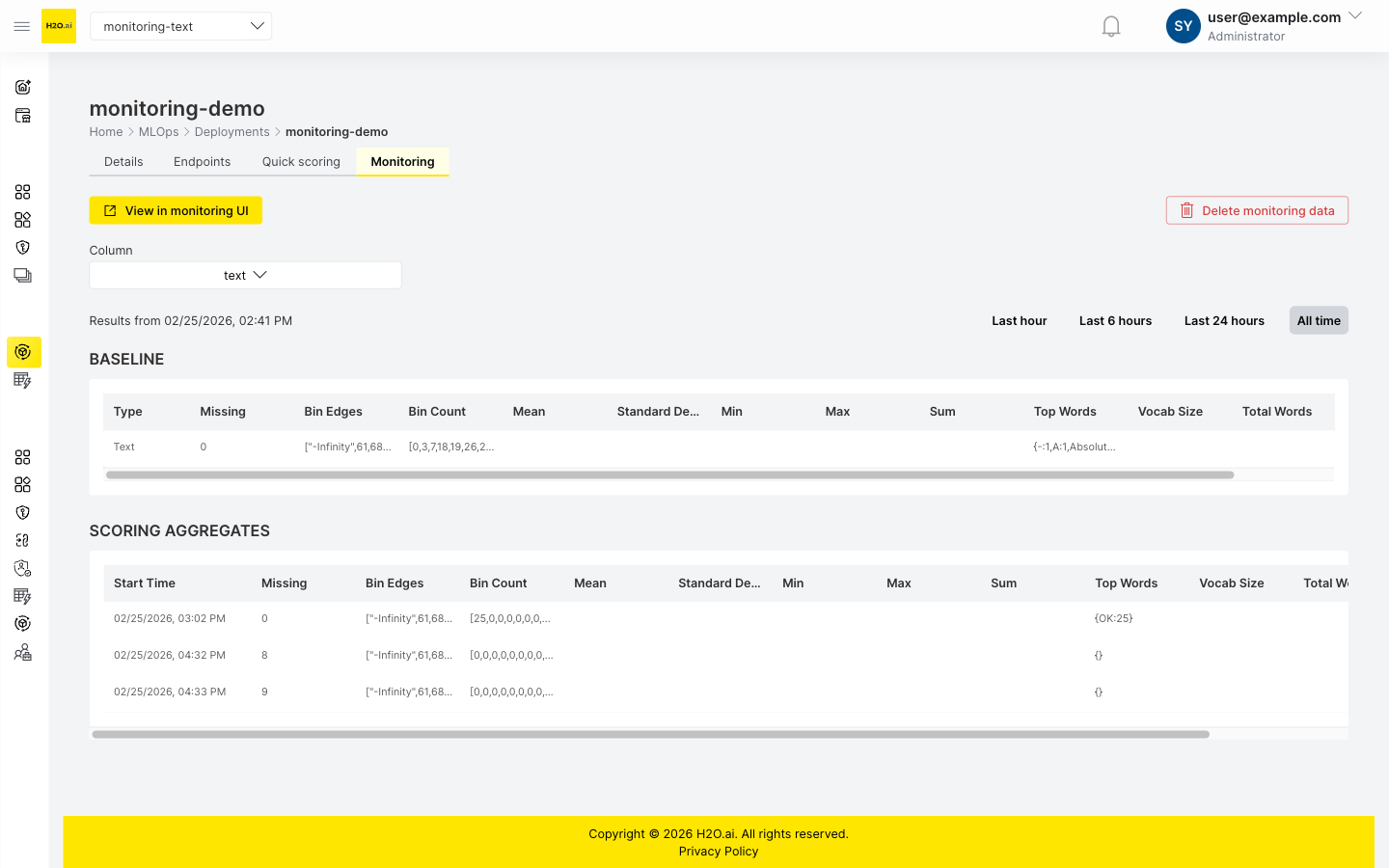
The monitoring tab summary table displays bin distributions and top words for text columns. For detailed length statistics (mean, standard deviation, min, max, sum) and vocabulary metrics (vocab size, total words), expand the baseline aggregation detail in the deployment's Monitoring options on the Details tab.

Key concepts for text monitoring

Text length bins (edges)

For TEXT features, H2O MLOps does not track the raw text values. Instead, it creates a histogram of text lengths and uses the histogram bins to detect distribution shifts over time. Each bin boundary in this histogram is called an edge. Edges are numeric boundaries; the ranges of character lengths between consecutive edges are the bins. The system stores only these boundaries and counts—not the text content itself.

Why track length instead of content?

• Scalability: Storing all unique text values is impractical for large datasets.
• Efficiency: Length histograms are compact and fast to compute.
• Drift detection: Shifts in the length distribution often indicate changes in the underlying text content.
• Privacy: The monitoring database does not need to store the actual text content.

Metrics collected for text columns

For each TEXT column, H2O MLOps computes two groups of statistics.

Length distribution

• Minimum, maximum, mean, sum, and standard deviation of character length.
• Histogram with quantile-based bins that adapt to the data.
• Counts of missing values and empty strings.

Vocabulary analysis

• Baseline vocabulary: The 100 most common words from the training data (fixed cap).
• Scoring vocabulary: Adaptive selection of top words that cover approximately 80% of text occurrences (minimum 50, maximum 1,000 words).
• Total vocabulary size (number of unique words).
• Total word count.
• Out-of-vocabulary (OOV) rate (scoring data only; see note below).

info

The OOV rate is only calculated for scoring rows. Baseline rows store oov_rate as NULL in the database because the baseline vocabulary is the reference itself — by definition, there are no out-of-vocabulary words at baseline time. The UI may display this value as 0. The SQL queries in this guide filter with AND oov_rate IS NOT NULL to exclude baseline rows from OOV analysis.

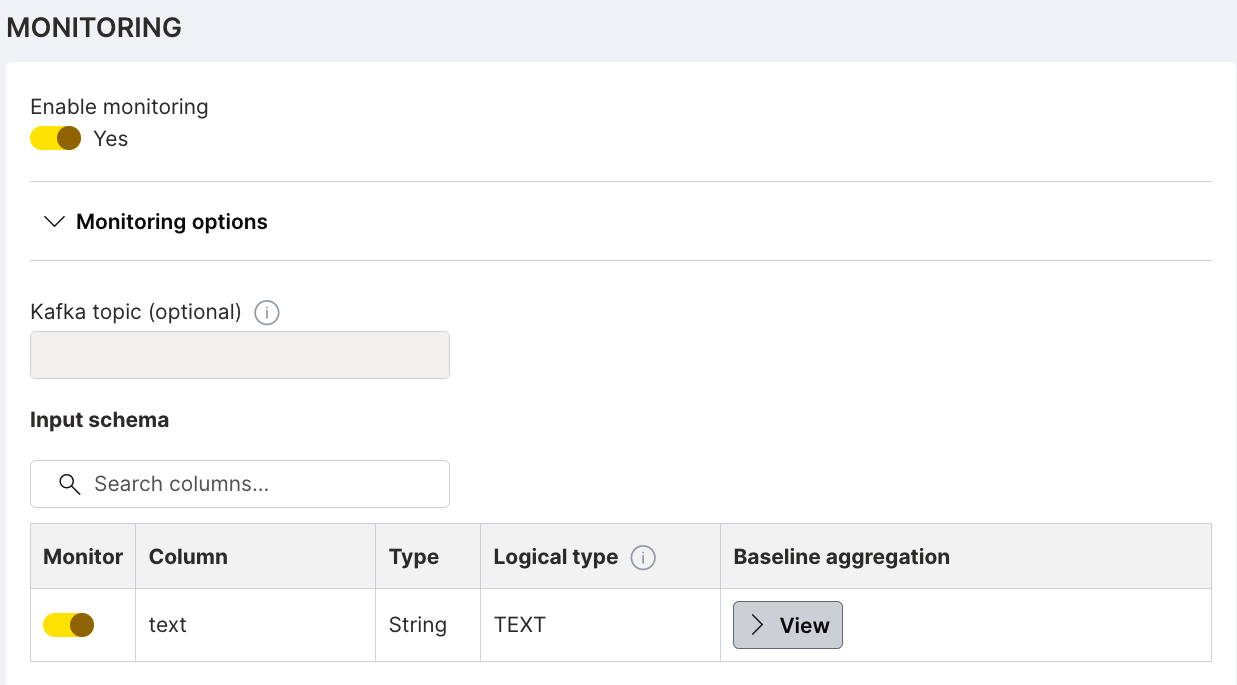
In the deployment's Monitoring options, the input schema table shows each monitored column with its type, logical type, and baseline aggregation. The following screenshot shows a text column configured with the TEXT logical type:

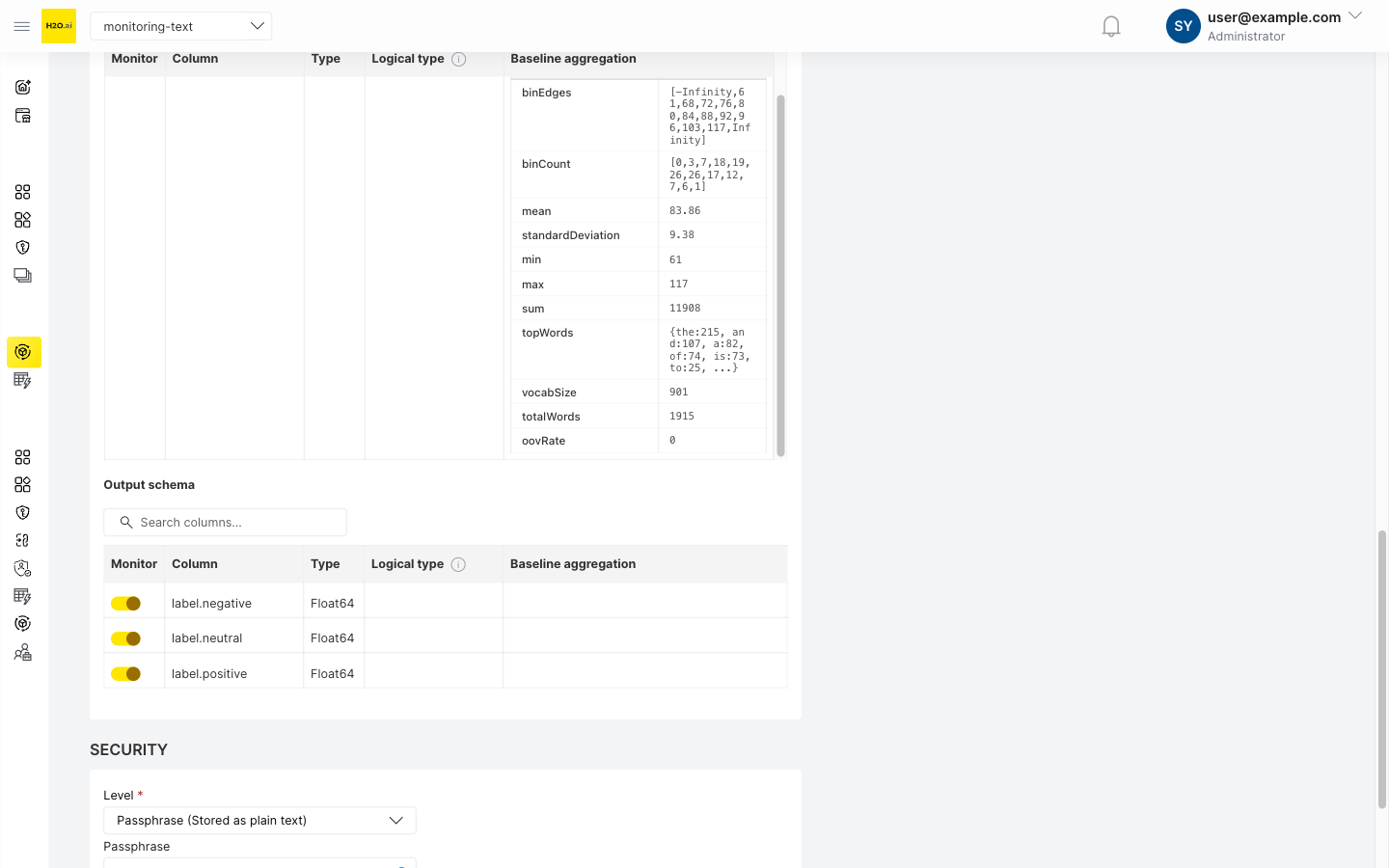
Click View to expand the baseline aggregation detail and inspect the stored metrics:

How text edges are calculated

Example 1: Simple text dataset

Sample data

texts = [
    "Hi",                                      # length: 2
    "Hello",                                   # length: 5
    "Good morning",                            # length: 12
    "How are you?",                            # length: 12
    "This is a longer text",                   # length: 22
    "Short",                                   # length: 5
    "Medium length text",                      # length: 18
    "Very long text that goes on and on",      # length: 36
]

# Extracted lengths
lengths = [2, 5, 12, 12, 22, 5, 18, 36]

Step 1: Calculate quantiles

H2O MLOps uses 10 bins (11 edges) by default, calculated at these percentiles:

probabilities = [0.0, 0.1, 0.2, 0.3, 0.4, 0.5, 0.6, 0.7, 0.8, 0.9, 1.0]

# Quantiles of the lengths
quantiles = [2, 5, 5, 8.4, 12, 12, 15, 18, 22, 29, 36]
# Interpretation:
#   0% (min) = 2 characters
#   50% (median) = 12 characters
#   100% (max) = 36 characters

# Remove duplicate values
unique_quantiles = [2, 5, 8.4, 12, 15, 18, 22, 29, 36]

Step 2: Add infinity boundaries

edges = [-inf, 2, 5, 8.4, 12, 15, 18, 22, 29, 36, +inf]

This creates the following bins:

Bin	Range	Description
1	(-inf, 2]	Empty or very short texts
2	(2, 5]	Very short (2-5 chars)
3	(5, 8.4]	Short (5-8 chars)
4	(8.4, 12]	Medium-short (8-12 chars)
5	(12, 15]	Medium (12-15 chars)
6	(15, 18]	Medium-long (15-18 chars)
7	(18, 22]	Long (18-22 chars)
8	(22, 29]	Very long (22-29 chars)
9	(29, 36]	Extra long (29-36 chars)
10	(36, +inf)	Extremely long texts

Step 3: Create histogram

Count how many texts fall into each bin:

Bin 1:  (-inf, 2]     → 0 texts
Bin 2:  (2, 5]        → 3 texts ("Hi"=2, "Hello"=5, "Short"=5)
Bin 3:  (5, 8.4]      → 0 texts
Bin 4:  (8.4, 12]     → 2 texts ("Good morning"=12, "How are you?"=12)
Bin 5:  (12, 15]      → 0 texts
Bin 6:  (15, 18]      → 1 text ("Medium length text"=18)
Bin 7:  (18, 22]      → 1 text ("This is a longer text"=22)
Bin 8:  (22, 29]      → 0 texts
Bin 9:  (29, 36]      → 1 text ("Very long text..."=36)
Bin 10: (36, +inf)    → 0 texts

Example 2: Real-world product reviews

This example demonstrates how drift detection works by comparing baseline (training) data against scoring (production) data.

Baseline data (training phase)

# 1000 product reviews from training data
baseline_lengths = [
    45, 67, 89, 123, 156, 178, 198, 234, 267, 289, ...
]
# Most reviews are 50-200 characters

# Calculate quantiles (10 bins)
baseline_quantiles = [10, 45, 67, 89, 112, 145, 178, 210, 245, 289, 450]

# Edges with infinities
baseline_edges = [-inf, 10, 45, 67, 89, 112, 145, 178, 210, 245, 289, 450, +inf]

# Baseline histogram (counts per bin)
baseline_counts = [2, 98, 123, 145, 156, 167, 134, 89, 56, 23, 7, 0]
#                  ^                     ^
#                  Few very short       Most reviews in middle bins (67-210 chars)

Length Distribution (Baseline)

 200|                  ##
 180|                  ##
 160|              ##  ##  ##
 140|          ##  ##  ##  ##
 120|      ##  ##  ##  ##  ##
 100|  ##  ##  ##  ##  ##  ##
  80|  ##  ##  ##  ##  ##  ##  ##
  60|  ##  ##  ##  ##  ##  ##  ##  ##
  40|  ##  ##  ##  ##  ##  ##  ##  ##  ##
  20|  ##  ##  ##  ##  ##  ##  ##  ##  ##  ##
   0|  ##  ##  ##  ##  ##  ##  ##  ##  ##  ##  ##  ##
     -------------------------------------------------
      <10 45  67  89  112 145 178 210 245 289 450 >450
                    Character Length Bins

Scoring data (after 1 month)

# New reviews coming in - users now writing much longer reviews!
scoring_lengths = [
    234, 345, 456, 567, 678, 789, 890, 234, 456, ...
]

# Use SAME baseline edges for comparison (crucial for drift detection)
scoring_edges = baseline_edges  # [-inf, 10, 45, 67, ..., 450, +inf]

# Scoring histogram (using baseline bins)
scoring_counts = [1, 45, 67, 89, 78, 98, 156, 189, 234, 123, 89, 45]
#                                            ^    ^    ^    ^   ^
#                       More reviews now in higher bins -> DRIFT DETECTED!

Length Distribution (Scoring)

 250|                                  ##
 230|                                  ##
 210|                              ##  ##
 190|                          ##  ##  ##
 170|                      ##  ##  ##  ##
 150|                  ##  ##  ##  ##  ##
 130|              ##  ##  ##  ##  ##  ##
 110|          ##  ##  ##  ##  ##  ##  ##  ##
  90|      ##  ##  ##  ##  ##  ##  ##  ##  ##  ##
  70|  ##  ##  ##  ##  ##  ##  ##  ##  ##  ##  ##  ##
  50|  ##  ##  ##  ##  ##  ##  ##  ##  ##  ##  ##  ##
   0|  ##  ##  ##  ##  ##  ##  ##  ##  ##  ##  ##  ##
     -------------------------------------------------
      <10 45  67  89  112 145 178 210 245 289 450 >450
                    Character Length Bins

DRIFT DETECTED: Distribution shifted toward longer reviews!

Score the deployment

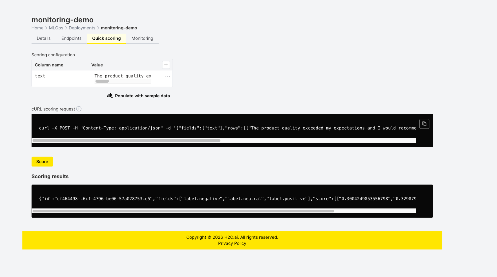
After deploying with monitoring enabled, score the deployment so that H2O MLOps can collect scoring data. On the Quick scoring tab, enter a text value in the Value field for the text column and click Score. The following screenshot shows the Quick scoring tab with a sample text entered and the scoring result:

After scoring, wait 3–5 minutes for aggregates to appear on the Monitoring tab.

SQL-based drift detection

This section provides ready-to-use SQL queries for detecting drift in text features directly in PostgreSQL. The queries run on the monitoring aggregates table that backs the Superset monitoring UI.

note

Replace <TABLE_NAME> in the queries below with your monitoring table name (for example, workspace_123.aggregates_deployment_id). For instructions on finding your schema and table name, see Analyze data in the monitoring UI.

All queries below analyze all text columns (logical_type = 4) for the deployment at once. This design provides:

• Unified dashboard: See drift across all text features in a single query.
• Efficient scanning: Scan the monitoring table once for all columns.
• Comparative analysis: Compare drift severity across different text columns.
• Batch monitoring: Process all text columns together for alerting.

To focus on a single column, add AND column_name = '<COLUMN_NAME>' to the WHERE clause, or filter the results client-side.

The following screenshot shows the OOV rate drift detection query in Superset SQL Lab. When scoring data with OOV metrics is available, the query returns rows with a drift_severity classification (for example, SEVERE, HIGH, or LOW):

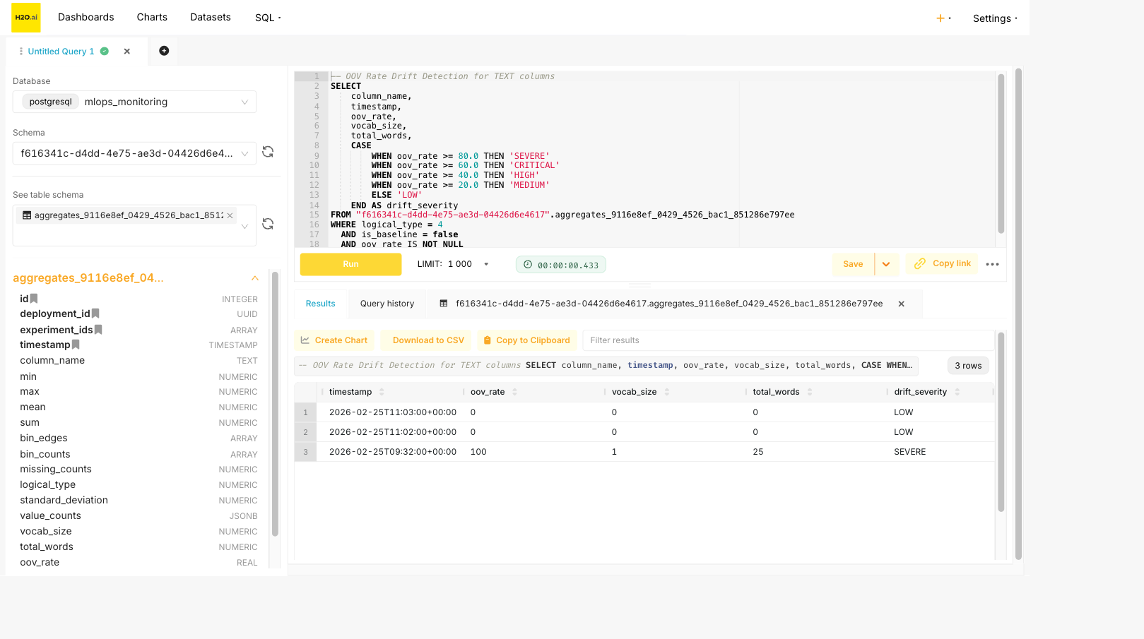
OOV rate drift detection

Detect vocabulary drift for all TEXT columns by comparing OOV rates over time.

-- Find scoring aggregates with high OOV rates across all TEXT columns
SELECT
    column_name,
    timestamp,
    oov_rate,
    vocab_size,
    total_words,
    CASE
        WHEN oov_rate >= 80.0 THEN 'SEVERE'
        WHEN oov_rate >= 60.0 THEN 'CRITICAL'
        WHEN oov_rate >= 40.0 THEN 'HIGH'
        WHEN oov_rate >= 20.0 THEN 'MEDIUM'
        ELSE 'LOW'
    END AS drift_severity
FROM <TABLE_NAME>
WHERE logical_type = 4
  AND is_baseline = false
  AND oov_rate IS NOT NULL
ORDER BY column_name, timestamp DESC;

OOV rate drift interpretation:

OOV Rate	Severity	Interpretation
0-20%	LOW	Normal vocabulary variation
20-40%	MEDIUM	Notable new vocabulary appearing
40-60%	HIGH	Significant vocabulary shift
60-80%	CRITICAL	Major vocabulary change
80-100%	SEVERE	Almost entirely new vocabulary

Time-series OOV trend analysis

Track OOV rate changes over time with moving averages for all TEXT columns.

-- Calculate 7-period moving average for OOV rate across all TEXT columns
WITH scoring_data AS (
    SELECT
        timestamp,
        column_name,
        oov_rate,
        vocab_size,
        total_words
    FROM <TABLE_NAME>
    WHERE logical_type = 4
      AND is_baseline = false
      AND oov_rate IS NOT NULL
    ORDER BY column_name, timestamp
),
windowed_stats AS (
    SELECT
        timestamp,
        column_name,
        oov_rate,
        AVG(oov_rate) OVER (
            PARTITION BY column_name
            ORDER BY timestamp
            ROWS BETWEEN 6 PRECEDING AND CURRENT ROW
        ) AS oov_rate_ma7,
        STDDEV(oov_rate) OVER (
            PARTITION BY column_name
            ORDER BY timestamp
            ROWS BETWEEN 6 PRECEDING AND CURRENT ROW
        ) AS oov_rate_stddev
    FROM scoring_data
)
SELECT
    column_name,
    timestamp,
    oov_rate,
    ROUND(oov_rate_ma7::numeric, 2) AS oov_rate_moving_avg,
    ROUND(oov_rate_stddev::numeric, 2) AS oov_rate_std,
    CASE
        WHEN oov_rate > oov_rate_ma7 + (2 * oov_rate_stddev) THEN 'ANOMALY_HIGH'
        WHEN oov_rate < oov_rate_ma7 - (2 * oov_rate_stddev) THEN 'ANOMALY_LOW'
        ELSE 'NORMAL'
    END AS anomaly_status
FROM windowed_stats
WHERE oov_rate_stddev IS NOT NULL
ORDER BY column_name, timestamp DESC;

Length distribution drift (chi-square test)

Compare the scoring histogram to the baseline using the chi-square statistic for all TEXT columns.

-- Chi-square test for histogram drift across all TEXT columns
WITH baseline AS (
    SELECT
        column_name,
        bin_edges,
        bin_counts
    FROM <TABLE_NAME>
    WHERE logical_type = 4
      AND is_baseline = true
),
scoring_aggregates AS (
    SELECT
        id,
        timestamp,
        column_name,
        bin_counts
    FROM <TABLE_NAME>
    WHERE logical_type = 4
      AND is_baseline = false
),
chi_square_calc AS (
    SELECT
        s.id,
        s.timestamp,
        s.column_name,
        s.bin_counts AS scoring_counts,
        b.bin_counts AS baseline_counts,
        array_length(s.bin_counts, 1) AS num_bins,
        (
            SELECT SUM(
                CASE
                    WHEN b.bin_counts[i] > 0 THEN
                        ((s.bin_counts[i] - b.bin_counts[i]) * (s.bin_counts[i] - b.bin_counts[i]))::numeric
                        / b.bin_counts[i]
                    ELSE 0
                END
            )
            FROM generate_series(1, array_length(s.bin_counts, 1)) AS i
        ) AS chi_square_statistic
    FROM scoring_aggregates s
    INNER JOIN baseline b ON s.column_name = b.column_name
)
SELECT
    column_name,
    timestamp,
    ROUND(chi_square_statistic, 4) AS chi_square,
    num_bins - 1 AS degrees_of_freedom,
    CASE
        WHEN chi_square_statistic > 21.666 THEN 'SIGNIFICANT (p < 0.01)'
        WHEN chi_square_statistic > 16.919 THEN 'SIGNIFICANT (p < 0.05)'
        WHEN chi_square_statistic > 14.684 THEN 'MARGINAL (p < 0.10)'
        ELSE 'NOT SIGNIFICANT'
    END AS drift_result
FROM chi_square_calc
ORDER BY column_name, timestamp DESC;

note

The critical values above assume 10 bins (9 degrees of freedom). Adjust thresholds for different bin counts:

Degrees of Freedom	p < 0.10	p < 0.05	p < 0.01
9	14.684	16.919	21.666
10	15.987	18.307	23.209
11	17.275	19.675	24.725

Mean length shift detection

Detect significant changes in mean text length using the z-score for all TEXT columns.

-- Mean length shift detection across all TEXT columns
WITH baseline AS (
    SELECT
        column_name,
        mean AS baseline_mean,
        standard_deviation AS baseline_std
    FROM <TABLE_NAME>
    WHERE logical_type = 4
      AND is_baseline = true
),
scoring_stats AS (
    SELECT
        timestamp,
        column_name,
        mean AS scoring_mean,
        standard_deviation AS scoring_std,
        min,
        max
    FROM <TABLE_NAME>
    WHERE logical_type = 4
      AND is_baseline = false
)
SELECT
    s.column_name,
    s.timestamp,
    ROUND(b.baseline_mean::numeric, 2) AS baseline_mean,
    ROUND(s.scoring_mean::numeric, 2) AS scoring_mean,
    ROUND((s.scoring_mean - b.baseline_mean)::numeric, 2) AS mean_shift,
    ROUND(
        (ABS(s.scoring_mean - b.baseline_mean) / NULLIF(b.baseline_std, 0))::numeric,
        2
    ) AS z_score,
    CASE
        WHEN ABS(s.scoring_mean - b.baseline_mean) / NULLIF(b.baseline_std, 0) > 3.0 THEN 'CRITICAL'
        WHEN ABS(s.scoring_mean - b.baseline_mean) / NULLIF(b.baseline_std, 0) > 2.0 THEN 'HIGH'
        WHEN ABS(s.scoring_mean - b.baseline_mean) / NULLIF(b.baseline_std, 0) > 1.5 THEN 'MODERATE'
        ELSE 'NORMAL'
    END AS drift_severity
FROM scoring_stats s
INNER JOIN baseline b ON s.column_name = b.column_name
ORDER BY s.column_name, s.timestamp DESC;

Vocabulary size drift

Track vocabulary expansion or contraction over time for all TEXT columns.

-- Vocabulary size change detection across all TEXT columns
WITH baseline AS (
    SELECT
        column_name,
        vocab_size AS baseline_vocab_size,
        total_words AS baseline_total_words
    FROM <TABLE_NAME>
    WHERE logical_type = 4
      AND is_baseline = true
),
scoring_vocab AS (
    SELECT
        timestamp,
        column_name,
        vocab_size AS scoring_vocab_size,
        total_words AS scoring_total_words
    FROM <TABLE_NAME>
    WHERE logical_type = 4
      AND is_baseline = false
)
SELECT
    s.column_name,
    s.timestamp,
    b.baseline_vocab_size,
    s.scoring_vocab_size,
    s.scoring_vocab_size - b.baseline_vocab_size AS vocab_size_change,
    ROUND(
        ((s.scoring_vocab_size::numeric - b.baseline_vocab_size) /
         NULLIF(b.baseline_vocab_size, 0)) * 100,
        2
    ) AS vocab_size_change_pct,
    ROUND(
        (s.scoring_vocab_size::numeric / NULLIF(s.scoring_total_words, 0)) * 100,
        2
    ) AS vocab_diversity_pct,
    CASE
        WHEN ABS(s.scoring_vocab_size - b.baseline_vocab_size)::numeric /
             NULLIF(b.baseline_vocab_size, 0) > 0.5 THEN 'HIGH'
        WHEN ABS(s.scoring_vocab_size - b.baseline_vocab_size)::numeric /
             NULLIF(b.baseline_vocab_size, 0) > 0.3 THEN 'MODERATE'
        ELSE 'LOW'
    END AS vocab_drift_level
FROM scoring_vocab s
INNER JOIN baseline b ON s.column_name = b.column_name
ORDER BY s.column_name, s.timestamp DESC;

---

Feedback

• Submit and view feedback for this page
• Send feedback about H2O MLOps to cloud-feedback@h2o.ai